Lecture 10 – the configuration model

I am aiming to write a short post about each lecture in my ongoing course on Random Graphs. Details and logistics for the course can be found here.

As we enter the final stages of the semester, I want to discuss some extensions to the standard Erdos-Renyi random graph which has been the focus of most of the course so far. Although we will not get far into the details during this course, the overall goal is to develop models which are close to Erdos-Renyi in terms of ease of analysis, while also allowing more of the features characteristic of networks observed in the real world.

One of the more obvious deficiencies of the sparse regime of Erdos-Renyi random graphs for modelling ‘real-world phenomena’ concerns the degree sequence. Indeed, the empirical degree distribution of G(n,c/n) converges to Poisson(c). By contrast, in real-world networks, a much wider range of degrees is typically observed, and in many cases it is felt that these should follow a power law, with a small number of a very highly connected agents.

One way around this problem to construct random graphs where we insist that the graph has a given sequence of degrees. The configuration model, which is the subject of this lecture and this post (and about which I’ve written before), offers one way to achieve this.

Definition and notes

Let and let be a sequence of non-negative integers such that is even. Then the configuration model with degree sequence d is a random multigraph with vertex set [n], constructed as follows:

• To each vertex , assign  half-edges;
• Then, take a uniform matching of these half-edges;
• Finally, for each pair of half-edges in the matching, replace the two half-edges with a genuine edge, to obtain the multigraph , in which, by construction, vertex i has degree .

One should note immediately that although the matching is uniform, the multigraph is not uniform amongst multigraphs with that degree sequence. Note also that the condition on the sums of the degrees is necessary for any graph, and in this context means that the number of half-edges is even, without which it would not be possible to construct a matching.

This effect is manifest in the simplest possible example, when n=2 and d=(3,3). There are two possible graphs, up to isomorphism, which are shown below:

For obvious reasons, we might refer to these as the handcuffs and the theta , respectively. It’s helpful if we, temporarily, assume the half-edges are distinguishable at the moment we join them up in the configuration model construction. Because then there are 3×3=9 ways to join them up to form the handcuffs (think of which half-edge ends up forming the edge between the two vertices) while there are 3!=6 ways to pair up the half-edges in the theta.

In general, for multigraphs H with the correct degree sequence, we have

where is the multiplicity with which a given edge e appears in H.

Note: it might seem counterintuitive that this procedure is biased against multiple edges and self-loops, but it is really just saying that there are more ways to form two distinct edges than to form two equal edges (ie a multiedge pair) when we view the half-edges as distinguishable. (See this post for further discussion of this aspect in the 3-regular setting.)

However, a consequence of this result is that if we condition on the event that is simple, then the resulting random graph is uniform on the set of simple graphs satisfying the degree property. Note that the same example as above shows that there’s no guarantee that there exists a simple graph whose degrees are some given sequence.

d-regular configuration model

In general, from a modelling point of view, we are particularly interested in simple, connected graphs, and so it is valuable to study whether the large examples of the configuration model are likely to have these properties. In this lecture, I will mainly focus on the case where the multigraphs are d-regular, meaning that all the vertices have degree equal to d. For the purposes of this lecture, we denote by , the d-regular configuration model .

• d=1: to satisfy the parity condition on the sums of degrees, we must have n even. But then will consist of n/2 disjoint edges.
• d=2: will consist of some number of disjoint cycles, and it is a straightforward calculation to check that when n is large, with high probability the graph will be disconnected.

In particular, I will focus on the case when d=3, which is the first interesting case. Most of the results we prove here can be generalised (under various conditions) to more general examples of the configuration model. The main goal of the lecture is revision of some techniques of the course, plus one new one, in a fresh setting, and the strongest possible versions of many of these results can be found amongst the references listed at the end.

Connectedness

In the lecture, we showed that is connected with high probability. This is, in fact, a very weak result, since in fact is d-connected with high probability for [Bol81, Wor81]. Here, d-connected means that one must remove at least d vertices in order to disconnect the graph, or, equivalently, that there are d disjoint paths between any pair of vertices. Furthermore, Bollobas shows that for , is a (random) expander family [Bol88].

Anyway, for the purposes of this course, the main tool is direct enumeration. The matching number satisfies

and so Stirling’s approximation gives the asymptotics

although it will be useful to use the true bounds

instead in some places. Anyway, in , there are 6n half-edges in total, and so the probability that the graph may be split into two parts consisting of vertices, with , and with no edges between the classes is

Kernels of critical graph components

This post is motivated by G(N,p), the classical Erdos-Renyi random graph, specifically its critical window, when .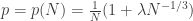

We start with the following observation, which makes no restriction on p. Suppose a component of G(N,p) is a tree. Then, the graph geometry of this component is that of a uniform random tree on the appropriate number of vertices. This is deliberately informal. To be formal, we’d have to say “condition on a particular subset of vertices forming a tree-component” and so on. But the formality is broadly irrelevant, because at the level of metric scaling limits, if we want to describe the structure of a tree component, it doesn’t matter whether it has or vertices, because in both cases the tree structure is uniform. The only thing that changes is the scaling factor.

In general, when V vertices form a connected component of a graph with E edges, we define the excess to be E-V+1. So the excess is non-negative, and is zero precisely when the component is a tree. I’m reluctant to say that the excess counts the number of cycles in the component, but certainly it quantifies the amount of cyclic structure present. We will sometimes, in a mild abuse of notation, talk about excess edges. But note that for a connected component with positive excess, there is a priori no way to select which edges would be the excess edges. In a graph process, or when there is some underlying exploration of the component, there sometimes might be a canonical way to classify the excess edges, though it’s worth remarking that the risk of size-biasing errors is always extremely high in this sort of situation.

Returning to the random graph process, as so often there are big changes around criticality. In the subcritical regime, the components are small, and most of them, even the largest with high probability, are trees. In the supercritical regime, the giant component has excess , which is qualitatively very different.

It feels like every talk I’ve ever given has begun with an exposition of Aldous’s seminal paper [Al97] giving a distributional scaling limit of the sizes of critical components in the critical window, and a relation between the process on this time-scale and the multiplicative coalescent. And it remains relevant here, because the breadth-first exploration process can also be used to track the number of excess edges.

In a breadth-first exploration, we have a stack of vertices we are waiting to explore. We pick one and look its neighbours restricted to the rest of the graph, that is without the vertices we have already fully explored, and also without the other vertices in the stack. That’s the easiest way to handle the total component size. But we can simultaneously track how many times we would have joined to a neighbour within the stack, which leads to an excess edge, and Aldous derives a joint distributional scaling limit for the sizes of the critical components and their excesses. (Note that in this case, there is a canonical notion of excess edge, but it depends not just on the graph structure, but also on the extra randomness of the ordering within the breadth-first search.)

Roughly speaking, we consider the reflected exploration process, and its scaling limit, which is a reflected parabolically-drifting Brownian motion (though the details of this are not important at this level of exposition, except that it’s a well-behaved non-negative process that hits zero often). The component sizes are given by the widths of the excursions above zero, scaled up in a factor . Then conditional on the shape of the excursion, the excess is Poisson with parameter the area under the excursion, with no rescaling. That is, a critical component has excess.

So, with Aldous’s result in the background, when we ask about the metric structure of these critical components, we are really asking: “what does a uniformly-chosen connected component with fixed excess look like when the number of vertices grows?”

I’ll try to keep notation light, but let’s say T(n,k) is a uniform choice from connected graphs on n vertices with excess k.

[Note, the separation of N and n is deliberate, because in the critical window, the connected components have size , so I want to distinguish the two problems.]

In this post, we will mainly address the question: “what does the cycle structure of T(n,k) look like for large n?” When k=0, we have a uniform tree, and the convergence of this to the Brownian CRT is now well-known [CRT2, LeGall]. We hope for results with a similar flavour for positive excess k.

2-cores and kernels

First, we have to give a precise statement of what it means to study just the cycle structure of a connected component. From now on I will assume we are always working with a connected graph.

There are several equivalent definitions of the 2-core C(G) of a graph G:

• When the excess is positive, there are some cycles. The 2-core is the union of all edges which form part of some cycle, and any edges which lie on a path between two edges which both form part of some cycle.
• C(G) is the maximal induced subgraph where all degrees are at least two.
• If you remove all the leaves from the graph, then all the leaves from the remaining graph, and continue, the 2-core is the state you arrive at where there are no leaves.

It’s very helpful to think of the overall structure of the graph as consisting of the 2-core, with pendant trees ‘hanging off’ the 2-core. That is, we can view every vertex of the 2-core as the root of a (possibly size 1) tree. This is particular clear if we remove all the edges of the 2-core from the graph. What remains is a forest, with one tree for each vertex of the 2-core.

In general, the k-core is the maximal induced subgraph where all degrees are at least k. The core is generally taken to be something rather different. For this post (and any immediate sequels) I will never refer to the k-core for k>2, and certainly not to the traditional core. So I write ‘core’ for ‘2-core’.

As you can see in the diagram, the core consists of lots of paths, and topologically, the lengths of these paths are redundant. So we will often consider instead the kernel, K(G), which is constructed by taking the core and contracting all the paths between vertices of degree greater than 2. The resulting graph has minimal degree at least three. So far we’ve made no comment about the simplicity of the original graphs, but certainly the kernel need not be simple. It will regularly have loops and multiple edges. The kernel of the graph and core in the previous diagram is therefore this:

Kernels of critical components

To recap, we can deconstruct a connected graph as follows. It has a kernel, and each edge of the kernel is a path length of some length in the core. The rest of the graph consists of trees hanging off from the core vertices.

For now, we ask about the distribution of the kernel of a T(n,K). You might notice that the case k=1 is slightly awkward, as when the core consists of a single cycle, it’s somewhat ambiguous how to define the kernel. Everything we do is easily fixable for k=1, but rather than carry separate cases, we handle the case .

We first observe that fixing k doesn’t confirm the number of vertices or edges in the kernel. For example, both of the following pictures could correspond to k=3:

However, with high probability the kernel is 3-regular, which suddenly makes the previous post relevant. As I said earlier, it can introduce size-biasing errors to add the excess edges one-at-a-time, but these should be constant factor errors, not scaling errors. So imagine the core of a large graph with excess k=2. For the sake of argument, assume the kernel has the dumbbell / handcuffs shape. Now add an extra edge somewhere. It’s asymptotically very unlikely that this is incident to one of the two vertices with degree three in the core. Note it would need to be incident to both to generate the right-hand picture above. Instead, the core will gain two new vertices of degree three.

Roughly equivalently, once the size of the core is fixed (and large) we have to make a uniform choice from connected graphs of this size where almost every vertex has degree 2, and of the rest have degree 3 or higher. But the sum of the degrees is fixed, because the excess is fixed. If there are n vertices in the core, then there are more graphs where all the vertices have degree 2 or 3, than graphs where a vertex has degree at least 4. Let’s state this formally.

Proposition: The kernel of a uniform graph with n vertices and excess is, with high probability as , 3-regular.

This proved rather more formally as part of Theorem 7 of [JKLP], essentially as a corollary after some very comprehensive generating function setup; and in [LPW] with a more direct computation.

In the previous post, we introduced the configuration model as a method for constructing regular graphs (or any graphs with fixed degree sequence). We observe that, conditional on the event that the resulting graph is simple, it is in fact uniformly-distributed among simple graphs. When the graph is allowed to be a multigraph, this is no longer true. However, in many circumstances, as remarked in (1.1) of [JKLP], for most applications the configuration model measure on multigraphs is the most natural.

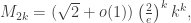
Given a 3-regular labelled multigraph H with 2(k-1) vertices and 3(k-1) edges, and K a uniform choice from the configuration model with these parameters, we have

where t(H) is the number of loops in H, and mult(e) the multiplicity of an edge e. This might seem initially counter-intuitive, because it looks we are biasing against graphs with multiple edges, when perhaps our intuition is that because there are more ways to form a set of multiple edges we should bias in favour of it.

I think it’s most helpful to look at a diagram of a multigraph as shown, and ask how to assign stubs to edges. At a vertex with degree three, all stub assignments are different, that is 3!=6 possibilities. At the multiple edge, however, we care which stubs match with which stubs, but we don’t care about the order within the multi-edge. Alternatively, there are three choices of how to divide each vertex’s stubs into (2 for the multi-edge, 1 for the rest), and then two choices for how to match up the multi-edge stubs, ie 18 in total = 36/2, and a discount factor of 2.

We mention this because in fact K(T(n,k)) converges in distribution to this uniform configuration model. Once you know that K(T(n,k)) is with high probability 3-regular, then again it’s probably easiest to think about the core, indeed you might as well condition on its total size and number of degree 3 vertices. It’s then not hard to convince yourself that a uniform choice induces a uniform choice of kernel. Again, let’s state that as a proposition.

Proposition: For any H a 3-regular labelled multigraph H with 2(k-1) vertices and 3(k-1) edges as before,

As we said before, the kernel describes the topology of the core. To reconstruct the graph, we need to know the lengths in the core, and then how to glue pendant trees onto the core. But this final stage depends on k only through the total length of paths in the core. Given that information, it’s a combinatorial problem, and while I’m not claiming it’s easy, it’s essentially the same as for the case with k=1, and is worth treating separately.

It is worth clarifying a couple of things first though. Even the outline of methods above relies on the fact that the size of the core diverges as n grows. Again, the heuristic is that up to size-biasing errors, T(n,k) looks like a uniform tree with some uniformly-chosen extra edges. But distances in T(n,k) scale like (and thus in critical components of G(N,p) scale like ). And the core will be roughly the set of edges on paths between the uniformly-chosen pairs of vertices, and so will also have length .

Once you have conditioned on the kernel structure, and the (large) number of internal vertices on paths in the core (ie the length of the core), it is natural that the assignment of the degree-2 vertices to core paths / kernel edges is uniform. A consequence of this is that if you record the lengths of paths in the core, where m=3(k-1), then

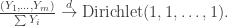
This is stated formally as Corollary 7 b) of [ABG09]. It’s worth noting that this confirms that the lengths of core paths are bounded in probability away from zero after the appropriate rescaling. In seeking a metric scaling limit, this is convenient as it means there’s so danger that two of the degree-3 vertices end up in ‘the same place’ in the scaling limit object.

To recap, the only missing ingredients now to give a complete limiting metric description of T(n,k) are 1) a distributional limit of the total core length; 2) some appropriate description of set of pendant trees conditional on the size of the pendant forest. [ABG09] show the first of these. As remarked before, all the content of the second of these is encoded in the unicyclic k=1 case, which I have written about before, albeit slightly sketchily, here. (Note that in that post we get around size-biasing by counting a slightly different object, namely unicyclic graphs with an identified cyclic edge.)

However, [ABG09] also propose an alternative construction, which you can think of as glueing CRTs directly onto the stubs of the kernel (with the same distribution as before). The proof that this construction works isn’t as painful as one might fear, and allows a lot of the other metric distributional results to be read off as corollaries.

References

[ABG09] – Addario-Berry, Broutin, Goldschmidt – Critical random graphs: limiting constructions and distributional properties

[CRT2] – Aldous – The continuum random tree: II

[Al97] – Aldous – Brownian excursions, critical random graphs and the multiplicative coalescent

[JKLP] – Janson, Knuth, Luczak, Pittel – The birth of the giant component

[LeGall] – Le Gall – Random trees and applications

[LPW] – Luczak, Pittel, Wierman – The structure of a random graph at the point of the phase transition

 

Random 3-regular graphs

A graph is d-regular if every vertex has degree d. Probably the easiest examples of d-regular graphs are the complete graph on (d+1) vertices, and the infinite d-ary tree. A less trivial example is the Petersen graph, which is 3-regular. 3-regular graphs will be the main focus for some of this post, but initially we lose nothing by considering general d.

Throughout, a necessary condition for the existence of a d-regular graph with N vertices is that at least one of d and N is even, as the sum of the degrees of a graph must be even. We will always assume that this holds, so that when d=3, we are always taking N to be even.

A natural pair of questions for a probabilist is ‘can we sample a d-regular graph with N vertices uniformly at random?’ and ‘what does a typical large d-regular graph look like?’

In a rather old post, I addressed some aspects of the first question, but revisit it briefly here. A good idea, due to Bollobas [B80] is to assign to all the vertices d stubs (or half-edges), and choose a matching of the Nd stubs uniformly at random. This works as a method to generate a random graph with any fixed degree sequence.

If you want your graphs to be simple, this can go wrong, because there’s a chance you get loops (that is, an edge from a vertex v to itself) and multiple edges between the same pair of vertices. It would be nice the graph formed in this fashion was simple with high probability when . Unfortunately that’s not the case, however the probability that the graph is simple remains asymptotically bounded away from 0 and 1. Indeed, because the presence of a loop / multiple edge is asymptotically independent of the presence of a loop / multiple edge elsewhere, it’s unsurprising we have a Poisson limit for the number of such occurences. So from a sampling point of view, it’s reasonable to sample a graph in this way until you find a simple one. This takes O(1) steps, and it’s O(N) steps to check whether a given multigraph is simple.

It’s clear that conditional on the graph generated in this fashion being simple, its distribution is uniform on the set of simple graphs with the correct degree distribution. If you are happy for your graphs to have loops, then it’s a little bit more complicated, because if an edge has multiplicity k, these can appear in k! ways in the configuration construction.

Other asymptotic properties

Loops and multiple edges can be thought of as cycles of length 1 and 2 respectively if you want. We might ask about other small cycles. A calculation in expectation is relatively straightforward. Given three vertices, the probability they form a triangle (in at least one way) is , and there are ways to choose three vertices. Thus the expected number of triangles is . Finally, the edge structure induced on disjoint triples is asymptotically independent, and hence a Poisson limit. (See [J06] for details, including more detail on the general configuration construction.) The same result holds for the same reasons for cycles of any fixed finite length.

We might also ask about connectivity. At a heuristic level, there are two ways for the graph to be disconnected: it could have some small components; or it could have two components of size . The smallest possible component is , and an argument like for the cycles above shows that the number of copies of vanishes in expectation. Now, consider having two components of size roughly N/2. There are ways to make this choice. However, given such a choice, we can handle the probability that all the stubs from one class match within that class by going through the class one stub at a time:

We approximate this as

and this dominates the number of choices powerfully enough that we might believe it remains valid for a broader range of class sizes. In fact we have a much stronger statement, namely that G(N,3) is 3-connected with high probability. This means that the graph cannot be disconnected by removing two vertices, or equivalently that there are three vertex-disjoint paths between any pair of vertices in the graph, essentially one emerging from each stub. See this note by David Ellis for a quick proof. We might return to this later.

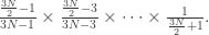
You might ask about planarity. It’s clear from degree consideration that there are no induced copies of in any random 3-regular graph, and since contains a cycle of length 4, and with high probability G(N,3) doesn’t, that takes care of that possibility too. However, there might be minors of this form. This seemed a good example of the Kuratowski criterion not actually being that useful, since I certainly don’t find the minors of the 3-regular graph an obvious structure to handle.

However, we can use Euler’s formula V – E + F = 2 for planar graphs. Here V = N, E = 3N/2. Faces are described by (a subset of the) cycles, and we there are asymptotically O(1) small cycles, so most faces include a large number of edges. But each edge corresponds to at most two faces. So we have , and so with high probability Euler’s formula can’t hold in G(N,3) for large N.

We can also ask about the local limit of G(N,3). Since the vertices are exchangeable, we don’t need to worry about whether we choose the root uniformly at random (often referred to as the Benjamini-Schramm sense) or by some other method.

The root has up to three neighbours, and with high probability it has exactly three neighbours. These neighbours have at most two other neighbours themselves. However, we’ve already seen that there are asymptotically O(1) cycles, and so with high probability there are no small cycles near a fixed root vertex. So the six neighbours-of-neighbours are with high probability different to the root and the root’s neighbours and to each other. We can make this argument at arbitrary finite radius from the root, to conclude that the local limit of G(N,3) is the infinite 3-ary tree.

Spectral expansion

[Caveat – this is something I read about and wanted to mention, but I really don’t know much at all about any of this theory, and it’s definitely not certain that what follows wouldn’t be better replaced by a set of links.]

This straightforward local limit offers good heuristics on some of the more global properties. Almost by definition, the d-ary tree expands as rapidly as is possible away from the root among infinite d-regular graphs. There are a number of ways to measure the expansion of a graph, and some methods transfer better to the infinite setting than others. The adjacency matrix of an infinite graph can be defined similarly to that of a finite graph, and it remains possible to talk about eigenfunctions and spectrum. As for the finite setting, d is an eigenvalue because the tree is d-regular, and -d is an eigenvalue because it is also bipartite.

The next largest eigenvalue governs the spectral gap which is a measure of the expansion of a graph. A graph is a good (spectral) expander if all the non-trivial eigenvalues are close to zero. A priori, all we know is that . For the infinite d-ary tree, we have . This blog post by Luca Trevisan gives a very readable proof.

A key result is that finite graphs can have , but not asymptotically. That is, taking N to be the number of vertices:

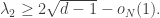
This is the content of the Alon-Boppana theorem [Al86]. In fact the error can be quantified as – the diamater of the graph is relevant here. A finite d-regular graph for which is called a Ramanujan graph. The existence of Ramanujan graphs has been much studied, and various constructions often rely on number theoretic properties of N, and lie at the interface of disparate branches of mathematics where my understanding is zero rather than epsilon.

Now return to our view of the d-ary tree as the local limit of a d-regular graph on N vertices for large N. We might expect from everything above that the uniform d-regular graph is a good expander. Bollobas shows that in the sense of edge-expansion, asymptotically almost all d-regular graphs have edge-expansion bounded away from zero. (See Section 2 of [Ell], including history of the d=3 case.) Friedman [Fri08] proves the conjecture of Alon that for every , a.a.s. for G(N,d) is at most . In this sense, G(N,d) is asymptotically ‘almost Ramanujan’. (See also [Bor17] for another proof and an introduction including history, context and references.)

Some other links: The Wikipedia page on expanders, which includes a discussion of the different descriptions of expansion, and the Cheeger inequalities and other relations between them; slides for a talk by Spielman on spectra and Ramanujan graphs; a survey by Murty on Ramanujan graphs;.

What next?

This post took a slightly different direction from what I had intended, and rather than make a halting U-turn back to my planned finale, I’ll postpone this. However, a short overture is that I’m interested in the structure of critical components of random graphs during the critical window. This is the window during which the largest components first have cycles with probability . Indeed, the critical components have size and  surplus edges. Conditional on their size, and number of surplus edges, the choice of the graph structure on the component is uniform among such (connected) graphs.

Addario-Berry, Broutin and Goldschmidt [ABG09] study scaling limits of such components. Central to this analysis is the 2-core of such components, which can be described in terms of 3-regular (multi)graphs. Various processes we are now interested in running on the critical components of critical RGs can then be studied in terms of related processes on random 3-regular graphs.

References

[ABG09] – Addario-Berry, Broutin, Goldschmidt – Critical random graphs: limiting constructions and distributional properties

[Al86] – Alon – Eigenvalues and expanders

[B80] – Bollobas – A probabilistic proof of an asymptotic formula for the number of labelled regular graphs

[B88] – Bollobas – The isoperimetric number of random regular graphs

[Bor17] – Bordenave – A new proof of Friedman’s second eigenvalue theorem and its extension to random lifts. Arxiv.

[Ell] – Ellis – The expansion of random regular graphs

[Fri08] – Friedman – A proof of Alon’s second eigenvalue conjecture and related problems

[J06] – Janson – The probability that a random multigraph is simple by