Antichains in the grid

Posted on February 6, 2017 by dominicyeo

In the previous post on this topic, we discussed Dilworth’s theorem on chains and antichains in a general partially ordered set. In particular, whatever the size of the largest antichain in a poset, it is possible to partition the poset into exactly that many chains. So for various specific posets, or the directed acyclic graphs associated to them, we are interested in the size of this largest antichain.

The following example turned out to be more interesting than I’d expected. At a conventional modern maths olympiad, there are typically three questions on each paper, and for reasons lost in the mists of time, each student receives an integer score between 0 and 7 per question. A natural question to ask is “how many students need to sit a paper before it’s guaranteed that one will scores at least as highly as another on every question?” (I’m posing this as a straight combinatorial problem – the correlation between scores on different questions will be non-zero and presumably positive, but that is not relevant here.)

The set of outcomes is clearly $\{0,1,\ldots,7\}^3$ , with the usual weak domination partial order inherited from $\mathbb{R}^3$ . Then an antichain corresponds to a set of triples of scores such that no triple dominates another triple. So the answer to the question posed is: “the size of the largest antichain in this poset, plus one.”

In general, we might ask about $\{1,2,\ldots,n\}^d$ , again with the weak domination ordering. This directed graph, which generalises the hypercube as well as our example, is called the grid.

Heuristics for the largest antichain

Retaining the language of test scores on multiple questions is helpful. In the previous post, we constructed a partition of the poset into antichains, indexed by the elements of some maximal chain, by starting with the sources, then looking at everything descended only from sources, and so on. (Recall that the statement that this is possible was referred to as the dual of Dilworth’s theorem.) In the grid, there’s a lot of symmetry (in particular under the mapping $x\mapsto n+1-x$ in every coordinate), and so you end up with the same family of antichains whether you work upwards from the sources or downwards from the sinks. (Or vice versa depending on how you’ve oriented your diagram…) The layers of antichains also have a natural interpretation – each layer corresponds to a given total score. It’s clear a priori why each of these is an antichain. If A scores the same as B overall, but strictly more on the first question, this must be counterbalanced by a strictly lower score on another question.

So a natural guess for the largest antichain is the largest antichain corresponding to some fixed total score. Which total score should this be? It ought to be the middle layer, that is total score $\frac{(n+1)d}{2}$ , or the two values directly on either side if this isn’t an integer. My intuition was probabilistic. The uniform distribution on the grid is achieved by IID uniform distributions in each coordinate, which you can think of as a random walk, especially if you subtract off the mean first. It feels that any symmetric random walk should have mode zero or next-to-zero. Certainly this works asymptotically in a rescaled sense by CLT, and in a slightly stronger sense by local CLT, but we don’t really want asymptotics here.

When I started writing the previous paragraph, I assumed there would be a simple justification for the claim that the middle layer(s) was largest, whether by straight enumeration, or some combinatorial argument, or even generating functions. Perhaps there is, and I didn’t spot it. Induction on d definitely works though, with a slightly stronger hypothesis that the layer sizes are symmetric around the median, and monotone on either side of the median. The details are simple and not especially interesting, so I won’t go into them.

From now on, the hypothesis is that this middle layer of the grid is the largest antichain. Why shouldn’t it, for example, be some mixture of middle-ish layers? (*) Well, heuristically, any score sequence in one layer removes several possibilities from a directly adjacent layer, and it seems unlikely that this effect is going to cancel out if you take some intermediate number of score sequences in the first layer. Also, the layers get smaller as you go away from the middle, so because of the large amount of symmetry (coordinates are exchangeable etc), it feels reasonable that there should be surjections between layers in the outward direction from the middle. The union of all these surjections gives a decomposition into chains.

This result is in fact true, and its proof by Bollobas and Leader, using shadows and compression can be found in the very readable Sections 0 and 1 of [1].

Most of the key ideas to a compression argument are present in the case n=2, for which some notes by Leader can be found here, starting with Proof 1 of Theorem 3, the approach of which is developed over subsequent sections. We treat the case n=2, but focusing on a particularly slick approach that does not generalise as successfully. We also return to the original case d=3 without using anything especially exotic.

Largest antichain in the hypercube – Sperner’s Theorem

The hypercube $\{0,1\}^d$ is the classical example. There is a natural correspondence between the vertices of the hypercube, and subsets of $[d]$ . The ordering on the hypercube corresponds to the ordering given by containment on $\mathcal{P}([d])$ . Almost by definition, the k-th layer corresponds to subsets of size k, and thus includes $\binom{d}{k}$ subsets. The claim is that the size of the largest antichain is $\binom{d}{\lfloor d/2 \rfloor}$ , corresponding to the middle layer if d is even, and one of the two middle layers if d is odd. This result is true, and is called Sperner’s theorem.

I know a few proofs of this from the Combinatorics course I attended in my final year at Cambridge. As explained, I’m mostly going to ignore the arguments using compression and shadows, even though these generalise better.

As in the previous post, one approach is to exhibit a covering family of exactly this number of disjoint chains. Indeed, this can be done layer by layer, working outwards from the middle layer(s). The tool here is Hall’s Marriage Theorem, and we verify the relevant condition by double-counting. Probably the hardest case is demonstrating the existence of a matching between the middle pair of layers when d is odd.

Take d odd, and let $d':= \lfloor d/2\rfloor$ . Now consider any subset S of the d’-th layer $\binom{[d]}{d'}$ . We now let the upper shadow of S be

$\partial^+(S):= \{A\in \binom{[d]}{d'+1}\,:\, \exists B\in S, B\subset A\},$

the sets in the (d’+1)-th layer which lie above some set in S. To apply Hall’s Marriage theorem, we have to show that $|\partial^+(S)|\ge |S|$ for all choice of S.

We double-count the number of edges in the hypercube from $S$ to $\partial^+(S)$ . Firstly, for every element $B\in S$ , there are exactly d’ relevant edges. Secondly, for every element $A\in\partial^+(S)$ , there are exactly d’ edges to some element of $\binom{[d]}{d'}$ , and so in particular there are at most d’ edges to elements of S. Thus

$d' |S|=|\text{edges }S\leftrightarrow\partial^+(S)| \le d' |\partial^+(S)|,$

which is exactly what we require for Hall’s MT. The argument for the matching between other layers is the same, with a bit more notation, but also more flexibility, since it isn’t a perfect matching.

The second proof looks at maximal chains. Recall, in this context, a maximal chain is a sequence $\mathcal{C}=B_0\subset B_1\subset\ldots\subset B_d$ where each $B_k:= \binom{[d]}{k}$ . We now consider some largest-possible antichain $\mathcal{A}$ , and count how many maximal chains include an element $A\in\mathcal{A}$ . If $|A|=k$ , it’s easy to convince yourself that there are $\binom{d}{r}$ such maximal chains. However, given $A\ne A'\in\mathcal{A}$ , the set of maximal chains containing A and the set of maximal chains containing A’ are disjoint, since $\mathcal{A}$ is an antichain. From this, we obtain

$\sum_{A\in\mathcal{A}} \binom{d}{|A|} \le d!.$ (**)

Normally after a change of notation, so that we are counting the size of the intersection of the antichain with each layer, this is called the LYM inequality after Lubell, Yamamoto and Meshalkin. The heuristic is that the sum of the proportions of layers taken up by the antichain is at most one. This is essentially the same as earlier at (*). This argument can also be phrased probabilistically, by choosing a *random* maximal chain, and considering the probability that it intersects the proposed largest antichain, which is, naturally, at most one. Of course, the content is the same as this deterministic combinatorial argument.

Either way, from (**), the statement of Sperner’s theorem follows rapidly, since we know that $\binom{d}{|A|}\le \binom{d}{\lfloor d/2\rfloor}$ for all A.

Largest antichain in the general grid

Instead of attempting a proof or even a digest of the argument in the general case, I’ll give a brief outline of why the previous arguments don’t transfer immediately. It’s pretty much the same reason for both approaches. In the hypercube, there is a lot of symmetry within each layer. Indeed, almost by definition, any vertex in the k-th layer can be obtained from any other vertex in the k-th layer just by permuting the labels (or permuting the coordinates if thinking as a vector).

The hypercube ‘looks the same’ from every vertex, but that is not true of the grid. Consider for clarity the n=8, d=3 case we discussed right at the beginning, and compare the scores (7,0,0) and (2,2,3). The number of maximal chains through (7,0,0) is $\binom{14}{7}$ , while the number of maximal chains through (2,2,3) is $\binom{7}{2, 2,3}\binom{14}{4,5,5}$ , and the latter is a lot larger, which means any attempt to use the second argument is going to be tricky, or at least require an extra layer of detail. Indeed, exactly the same problem arises when we try and use Hall’s condition to construct the optimal chain covering directly. In the double-counting section, it’s a lot more complicated than just multiplying by d’, as was the case in the middle of the hypercube.

Largest antichain in the d=3 grid

We can, however, do the d=3 case. As we will see, the main reason we can do the d=3 case is that the d=2 case is very tractable, and we have lots of choices for the chain coverings, and can choose one which is well-suited to the move to d=3. Indeed, when I set this problem to some students, an explicit listing of a maximal chain covering was the approach some of them went for, and the construction wasn’t too horrible to state.

[Another factor is that it computationally feasible to calculate the size of the middle layer, which is much more annoying in d>3.]

[I’m redefining the grid here as $\{0,1,\ldots,n-1\}^d$ rather than $\{1,2,\ldots,n\}^d$ .]

The case distinction between n even and n odd is going to make both the calculation and the argument annoying, so I’m only going to treat the even case, since n=8 was the original problem posed. I should be honest and confess that I haven’t checked the n odd case, but I assume it’s similar.

So when n is even, there are two middle layers namely $\frac{3n}{2}-2, \frac{3n}{2}-1$ (corresponding to total score 10 and total score eleven in the original problem). I calculated the number of element in the $\frac{3n}{2}-1$ layer by splitting based on the value of the first coordinate. I found it helpful to decompose the resulting sum as

$\sum_{k=0}^{n-1} = \sum_{k=0}^{\frac{n}{2}-1} + \sum_{k=\frac{n}{2}}^{n-1},$

based on whether there is an upper bound, or a lower bound on the value taken by the second coordinate. This is not very interesting, and I obtained the answer $\frac{3n^2}{4}$ , and of course this is an integer, since n is even.

Now to show that any antichain has size at most $\frac{3n^2}{4}$ . Here we use our good control on the chain coverings in the case d=2. We note that there is a chain covering of the (n,d=2) grid where the chains have 2n-1, 2n-3,…, 3, 1 elements (%). We get this by starting with a maximal chain, then taking a maximal chain on what remains etc. It’s pretty much the first thing you’re likely to try.

Consider an antichain with size A in the (n,d=3) grid, and project into the second and third coordinates. The image sets are distinct, because otherwise a non-trivial pre-image would be a chain. So we have A sets in the (n,d=2) grid. How many can be in each chain in the decomposition (%). Well, if there are more than n in any chain in (%), then two must have been mapped from elements of the (n,d=3) grid with the same first coordinate, and so satisfy a containment relation. So in fact there are at most n image points in any of the chains of (%). So we now have a bound of $n^2$ . But of course, some of the chains in (%) have length less than n, so we are throwing away information. Indeed, the number of images points in a given chain is at most

$\max(n,\text{length of chain}),$

and so the number of image points in total is bounded by

$n+\ldots+n+ (n-1)+(n-3)+\ldots+1,$

where there are n/2 copies of n in the first half of the sum. Evaluating this sum gives $\frac{3n^2}{4}$ , exactly as we wanted.

References

[1] – Bollobas, Leader (1991) – Compressions and Isoperimetric Inequalities. Available open-access here.

Enumerating Forests

Posted on February 16, 2015 by dominicyeo

I’ve just got back from a visit to Budapest University of Technology, where it was very pleasant to be invited to give a talk, as well as continuing the discussion our research programme with Balazs. My talk concerned a limit for the exploration process of an Erdos-Renyi random graph conditioned to have no cycles. Watch this space (hopefully very soon) for a fully rigorous account of this. In any case, my timings were not as slick as I would like, and I had to miss out a chunk I’d planned to say about a result of Britikov concerning enumerating unrooted forests. It therefore feels like an excellent time to write something again, and explain this paper, which you might be able to find here, if you have appropriate journal rights.

We are interested to calculate $a_{n,m}$ the number of forests with vertex set [n] consisting of m unrooted trees. Recall that if we were interested in rooted trees, we could appeal to Prufer codes to show that there are $m n^{n-m-1}$ such forests, and indeed results of Pitman give a coalescent/fragmentation scheme as m varies between 1 and n-1. It seems that there is no neat combinatorial re-interpretation of the unrooted case though, so Britikov uses an analytic method.

We know that

$a_{n,m}= \frac{n!}{m!} \sum_{\substack{k_1+\ldots+k_m=n\\ k_i\ge 1}} \prod_{j=1}^m \frac{k_j^{k_j-2}}{k_j!}.$

To see this, observe that the $k_j$ s correspond to the sizes of the m trees in the forest; $\frac{n!}{\prod k_j!}$ gives the multinomial number of ways to assign vertices to the trees; given the labels for a tree of size $k_j$ , there are $k_j^{k_j-2}$ ways to make up the tree itself; and $\frac{1}{m!}$ accounts for the fact that the trees have no order.

What we would really like to do is to take the uniform distribution on the set of all labelled trees, then simulate m IID copies of this distribution, and condition the union to contain precisely n vertices. But obviously this is an infinite set, so we cannot choose uniformly from it. Instead, we can tilt so that large trees are unlikely. In particular, for each x we define

$\mathbb{P}(\xi=k) \propto \frac{k^{k-2} x^k}{k!}$ ,

and define the normalising constant

$B(x):= \sum_{k\ge 1} \frac{k^{k-2}x^k}{k!},$

whenever it exists. It turns out that $x\le e^{-1}$ is precisely the condition for $B(x)<\infty$ . Note now that if $\xi_1,x_2,\ldots$ are IID copies of $\xi$ , then

$\mathbb{P}(\xi_1+\ldots+\xi_m=n) = \frac{x^n}{B(x)^m} \sum_{k_1+\ldots + k_m=n} \prod_{j=1}^m \frac{k_j^{k_j-2}}{k_j!},$

and so we obtain

$a_{n,m}= \frac{n!}{m!} \frac{B(x)^m}{x^n} \mathbb{P}(\xi_1+\ldots + \xi_m=n).$

So asymptotics for $a_{n,m}$ might follows from laws of large numbers of this distribution $\xi$ .

So far, we haven’t said anything about how to choose this value x. But observe that if you want to have lots of trees in the forest, then the individual trees should generally be small, so we take x small to tilt away from a preference for large trees. It turns out that there is a similar interpretation of criticality for forests as for general graphs, and taking x equal to 1/e, its radius of convergence works well for this setting. If you want even fewer trees, there is no option to take x larger than 1/e, but instead one can use large deviations machinery rather than laws of large number asymptotics.

We will be interested in asymptotics of the characteristic function of $\xi$ for x=1/e. In particular $\mathbb{E}[e^{it\xi}]=\frac{B(xe^{it})}{B(x)}$ , and it will be enough to clarify the behaviour of this as $t\rightarrow 0$ . It’s easier to work with a relation analytic function

$\theta(x)=\sum_{k\ge 1} \frac{k^{k-1}x^k}{k!},$

ie the integral of B. What now feels like a long time ago I wrote a masters’ thesis on the subject of multiplicative coalescence, and this shows up as the generating function of the solutions to Smoluchowski’s equations with monodisperse initial conditions, which are themselves closely related to the Borel distributions. In any case, several of the early papers on this topic made progress by establishing that the radius of convergence is 1/e, and that $\theta(x)e^{-\theta(x)}=x$ everywhere where $|x|\le 1/e$ . We want to consider x=1/e, for which $\theta=1$ .

Note that $\mathbb{E}\xi = \frac{\theta(x)}{B(x)}$ , so we will make progress by relating $B(x),\theta(x)$ in two ways. One way involves playing around with contour integrals in a fashion that is clear in print, but involves quite a lot of notation. The second way is the Renyi relation which asserts that $\theta(x)=B(x)+\frac{\theta(x)^2}{2}$ . We will briefly give a combinatorial proof. Observe that after multiplying through by factorials and interpreting the square of a generating function, this is equivalent to

$k^{k-1} = k^{k-2} + \frac12 \sum_{\substack{l+m=k\\l,m\ge 1}} l^{l-1}m^{m-1}\binom{k}{l},$

for all k. As we might expect from the appearance of this equality, we can prove it using a bijection on trees. Obviously on the LHS we have the size of the set of rooted trees on [k]. Now consider the set of pairs of disjoint rooted trees with vertex set [k]. This second term on the RHS is clearly the size of this set. Given an element of this set, join up the two roots, and choose whichever root was not initially in the same tree as 1 to be the new root. We claim this gives a bijection between this set, and the set of rooted trees on [k], for which 1 is not the root. Given the latter, the only pair of trees that leads to the right rooted tree on [k] under this mapping is given by cutting off the unique edge incident to the root that separates the root and vertex 1. In particular, since there is a canonical bijection between rooted trees for which 1 is the root, and unrooted trees (!), we can conclude the Renyi relation.

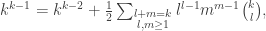
The Renyi relation now gives $\mathbb{E}\xi = \frac{\theta(x)}{B(x)}=2$ when x=1/e. If we wanted, we could show that the variance is infinite, which is not completely surprising, as the parameter x lies on the radius of convergence of the generating function.

Now, playing around with contour integrals, and being careful about which strands to take leads to the asymptotic as $t\rightarrow 0$

$\mathbb{E}[ e^{it\xi}] = 1+2it + \frac{2}{3}i |2t|^{3/2} (i\mathrm{sign}(t))^{3/2} + o(|t|^{3/2}).$

So from this, we can show that the characteristic function of the rescaled centred partial sum $\frac{\xi_1+\ldots+\xi_N-2N}{bN^{2/3}}$ converges to $\exp(-|t|^{3/2}\exp(\frac{i\pi}{4}\mathrm{sign} t))$ , where $b= (32/9)^{1/3}$ is a constant arising out of the previous step.

We recognise this as the characteristic function of the stable distribution with parameters 3/2 and -1. In particular, we know now that $\xi$ is in the domain of attraction for a stable-3/2 distribution. If we wanted a version of the central limit theorem for such partial sums, we could have that, but since we care about the partial sums of the $\xi_i$ s taking a specific value, rather than a range of values on the scale of the fluctuations, we actually need a local limit theorem.

To make this clear, let’s return to the simplest example of the CLT, with some random variables with mean $\mu$ and variance $\sigma^2<\infty$ . Then the partial sums satisfy

$\mathbb{P}(\mu N + a\sigma\sqrt{N} \le S_N \le \mu_N+b\sigma\sqrt{N}) \rightarrow \int_a^b f_{\mathcal N}(x)dx,$

as $N\rightarrow\infty$ . But what about the probability of $S_N$ taking a particular value m that lies between $\mu N+a\sigma \sqrt{N}$ and $\mu N + b\sigma \sqrt{N}$ ? If the underlying distribution was continuous, this would be uncontroversial – considering the probability of lying in a range that is smaller than the scale of the CLT can be shown in a similar way to the CLT itself. A local limit theorem asserts that when the underlying distribution is supported on some lattice, mostly naturally the integers, then these probabilities are in the limit roughly the same whenever m is close to $\mu N+a\sigma\sqrt{N}$ .

In this setting, a result of Ibragimov and Linnik that I have struggled to find anywhere in print (especially in English) gives us local limit theory for integer-supported distributions in the domain of attraction of a stable distribution. Taking p( ) to be the density of this distribution, we obtain

$bm^{2/3}\mathbb{P}(\xi_1+\ldots+\xi_m=n) - p(\frac{n-2m}{b m^{2/3}}) \rightarrow 0$

as $n\rightarrow\infty$ , uniformly on any set of m for which $z= \frac{n-2m}{bm^{2/3}}$ is bounded. Conveniently, the two occurrences of b clear, and Britikov obtains

$a_{n,m} = (1+o(1)) \frac{\sqrt{2\pi} n^{n-1/6}}{2^{n-m}(n-m)!} p(\frac{n-2m}{n^{2/3}},$

uniformly in the same sense as before.

Generating Functions for the IMO

Posted on April 16, 2013 by dominicyeo

The background to this post is that these days I find myself using generating functions all the time, especially for describing the stationary states of various coalescence-like processes. I remember meeting them vaguely while preparing for the IMO as a student. However, a full working understanding must have eluded me at the time, as for Q5 on IMO 2008 in Madrid I had written down in big boxes the two statements involving generating functions that immediately implied the answer, but failed to finish it off. The aim of this post is to help this year’s team avoid that particular pitfall.

What are they?

I’m going to define some things in a way which will be most relevant to the type of problems you are meeting now. Start with a sequence $(a_0,a_1,a_2,\ldots)$ . Typically these will be the sizes of various combinatorial sets. Eg a_n = number of partitions of [n] with some property. Define the generating function of the sequence to be:

$f(x)=\sum_{k\geq 0}a_k x^k=a_0+a_1x+a_2x^2+\ldots.$

If the sequence is finite, then this generating function is a polynomial. In general it is a power series. As you may know, some power series can be rather complicated, in terms of where they are defined. Eg

$1+x+x^2+x^3+\ldots=\frac{1}{1-x},$

only when |x|<1. For other values of x, the LHS diverges. Defining f over C is fine too. This sort of thing is generally NOT important for applications of generating functions to combinatorics. To borrow a phrase from Wilf, a generating function is a convenient `clothesline’ on which to hang a sequence of numbers.

We need a notation to get back from the generating function to the coefficients. Write $[x^k]g(x)$ to denote the coefficient of $x^k$ in the power series g(x). So, if $g(x)=3x^3-5x^2+7$ , then $[x^2]g(x)=-5$ . It hopefully should never be relevant unless you read some other notes on the topic, but the notation $[\alpha x^2]g(x):=\frac{[x^2]g(x)}{\alpha}$ , which does make sense after a while.

How might they be useful?

Example: binomial coefficients $a_k=\binom{n}{k}$ appear, as the name suggests, as coefficients of

$f_n(x)=(1+x)^n=\sum_{k=0}^n \binom{n}{k}x^k.$

Immediate consequence: it’s trivial to work out $\sum_{k=0}^n \binom{n}{k}$ and $\sum_{k=0}^n(-1)^k \binom{n}{k}$ by substituting $x=\pm 1$ into f_n.

Less obvious consequence. By considering choosing n from a red balls and b blue balls, one can verify

$\binom{a+b}{n}=\sum_{k=0}^n \binom{a}{k}\binom{b}{n-k}.$

We can rewrite the RHS as

$\sum_{k+l=n}\binom{a}{k}\binom{b}{l}.$

Think how we calculate the coefficient of $x^n$ in the product $f(x)g(x)$ , and it is now clear that $\binom{a+b}{n}=[x^n](1+x)^{a+b}$ , while

$\sum_{k+l=n}\binom{a}{k}\binom{b}{l}=[x^n](1+x)^a(1+x)^b,$

so the result again follows. This provides a good slogan for generating functions: they often replicate arguments via bijections, even if you can’t find the bijection.

Useful for? – Multinomial sums

The reason why the previous argument for binomial coefficients worked nicely is because we were interested in the coefficients, but had a neat expression for the generating function as a polynomial. In particular, we had an expression

$\sum_{k+l=n}a_k b_l.$

This is always a clue that generating functions might be useful. This is sometimes called a convolution.

Exercise: prove that in general, if f(x) is the generating function of (a_k) and g(x) the generating function of (b_l), then f(x)g(x) is the generating function of $\sum_{k+l=n}a_kb_l$ .

Even more usefully, this works in the multinomial case:

$\sum_{k_1+\ldots+k_m=n}a^{(1)}_{k_1}\ldots a^{(m)}_{k_m}.$

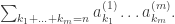
In many applications, these $a^{(i)}$ s will all be the same. We don’t even have to specify how many k_i’s there are to be considered. After all, if we want the sum to be n, then only finitely many can be non-zero. So:

$\sum_{m}\sum_{k_1+\ldots+k_m=n}a_{k_1}\ldots a_{k_m}=[x^n]f(x)^n=[x^n]f(x)^\infty,$

provided f(0)=1.

Useful when? – You recognise the generating function!

In some cases, you can identify the generating function as a `standard’ function, eg the geometric series. In that case, manipulating the generating functions is likely to be promising. Here is a list of some useful power series you might spot.

$1+x+x^2+\ldots=\frac{1}{1-x},\quad |x|<1$

$1+2x+3x^2+\ldots=\frac{1}{(1-x)^2},\quad |x|<1$

$e^x=1+x+\frac{x^2}{2!}+\frac{x^3}{3!}+\ldots$

$\cos x=1-\frac{x^2}{2!}+\frac{x^4}{4!}\pm\ldots$

Exercise: if you know what differentiation means, show that if f(x) is the gen fn of (a_k), then xf'(x) is the gen fn of ka_k.

Technicalities: some of these identities are defined only for certain values of x. This may be a problem if they are defined at, say, only a single point, but in general this shouldn’t be the case. In addition, you don’t need to worry about differentiability. You can definition differentiation of power series by $x^n\mapsto nx^{n-1}$ , and sort out convergence later if necessary.

Useful for? – Recurrent definitions

The Fibonacci numbers are defined by:

$F_0=F_1=1,\quad F_{n+1}=F_n+F_{n-1},\quad n\geq 1.$

Let F(x) be the generating function of the sequence F_n. So, for n=>1,

$[x^n]F(x)=[x^{n-1}]F(x)+[x^{n-2}]F(x)=[x^n](xF(x)+x^2F(x)),$

and F(0)=1, so we can conclude that:

$F(x)=1+(x+x^2)F(x)\quad\Rightarrow\quad F(x)=\frac{1}{1-x-x^2}.$

Exercise: Find a closed form for the generating function of the Catalan numbers, defined recursively by:

$C_n=C_0C_{n-1}+C_1C_{n-2}+\ldots+C_{n-1}C_0.$

Can you now find the coefficients explicitly for this generating function?

Useful for? – Partitions

Partitions can be an absolute nightmare to work with because of the lack of explicit formulae. Often any attempt at a calculation turns into a massive IEP bash. This prompts a search for bijective or bare-hands arguments, but generating functions can be useful too.

For now (*), let’s assume a partition of [n] means a sequence of positive integers $a_1\geq a_2\geq\ldots\geq a_k$ such that $a_1+\ldots+a_k=n$ . Let p(n) be the number of partitions of [n].

(* there are other definitions, in terms of a partition of the set [n] into k disjoint but unlabelled sets. Be careful about definitions, but the methods often extend to whatever framework is required. *)

Exercise: Show that the generating function of p(n) is:

$\left(\frac{1}{1-x}\right)\left(\frac{1}{1-x^2}\right)\left(\frac{1}{1-x^3}\right)\ldots$

Note that if we are interested only in partitions of [n], then we don’t need to consider any terms with exponent greater than n, so if we wanted we could take a finite product instead.

Example: the mint group will remember this problem from the first session in Cambridge:

Show that the number of partitions of [n] with distinct parts is equal to the number of partitions of [n] with odd parts.

Rather than the fiddly bijection argument found in the session, we can now treat this as a simple calculation. The generating function for distinct parts is given by:

$(1+x)(1+x^2)(1+x^3)\ldots,$

while the generating function for odd parts is given by:

$\left(\frac{1}{1-x}\right)\left(\frac{1}{1-x^3}\right)\left(\frac{1}{1-x^5}\right)\ldots.$

Writing the former as

$\left(\frac{1-x^2}{1-x}\right)\left(\frac{1-x^4}{1-x^2}\right)\left(\frac{1-x^6}{1-x^3}\right)\ldots$

shows that these are equal and the result follows.

Other things – Multivariate Generating Functions

If you want to track a sequence in two variables, say $a_{m,n}$ , then you can encode this with the bivariate generating function

$f(x,y):=\sum_{m,n\geq 0}a_{m,n}x^my^n.$

The coefficients are then extracted by $[x^ay^b]$ and so on. There’s some interesting stuff on counting lattice paths with this method.

Sums over arithmetic progressions via roots of unity

Note that we can extract both $\sum a_n$ and $\sum (-1)^na_n$ by judicious choice of x in f(x). By taking half the sum or half the difference, we can obtain

$a_0+a_2+a_4+\ldots=\frac12(f(1)+f(-1)),\quad a_1+a_3+a_5+\ldots=\frac12(f(1)-f(-1)).$

Can we do this in general? Yes actually. If you want $a_0+a_k+a_{2k}+\ldots$ , this is given by:

$a_0+a_k+a_{2k}+\ldots+\frac{1}{k}\left(f(1)+f(w)+\ldots+f(w^{k-1})\right),$

where $w=e^{2\pi i/k}$ is a $k$th root of unity. Exercise: Prove this.

For greater clarity, first try the case k=4, and consider the complex part of the power series evaluated at +i and -1.

Mutual information and moment generating functions (cs.stackexchange.com)
Generators functions only yields first item (stackoverflow.com)
Poisson Tails (eventuallyalmosteverywhere.wordpress.com)
Bell polynomials (eventuallyalmosteverywhere.wordpress.com)
Exponentials kill polynomials
Bijections etc.

Eventually Almost Everywhere

A blog about probability and olympiads by Dominic Yeo

Tag Archives: multinomial coefficients

Antichains in the grid

Enumerating Forests

Generating Functions for the IMO

Related articles