Queues and Migration Processes

Simple Queues

A queue generally has the form of a countable state-space Markov Chain. Here we assume that customers are served in the order they arrive (often referred to as: FIFO – First In First Out). The standard Kendall notation is M/M/C/K. Here the Ms stand for Markov (or memoryless) arrivals, and service times respectively, possibly replaced by G if the process admits more general distributions. C is the number of servers, and K the capacity of the system.

The first example is a M/M/C/C queue, motivated by a telephone network. Here, there are c lines, and an arriving call is lost if all lines are busy at the arrival time. We assume arrivals are a PP( $\lambda$ ) process, and the call times are iid Exp( $\mu$ ) RVs. We record the number of busy lines, which is a continuous-time Markov chain on state-space [0,c]. As usual, we assume the system operates in equilibrium, and so in particular we must have $\lambda<\mu c$ . It is easy to find the equilibrium distribution. The only non-zero transition probabilities are

$q(i-1,i)=\lambda, \quad q(i,i-1)=\mu i\quad i=1,\ldots,c$

and so can that that $\pi_i=\frac{\nu_i}{i!}\pi_0$ satisfies the DBEs where $\nu:=\frac{\lambda}{\mu}$ , sometimes called the traffic intensity. This gives

$\pi_c=\mathbb{P}(c\text{ lines busy})=\frac{\nu^c}{c!}\left(\sum_{k=0}^c \frac{\nu^k}{k!}\right)^{-1}$

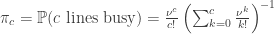
and we define this to be $E(\nu,c)$ , Erlang’s formula.

Note that if $(X(t),t\in\mathbb{R})$ is a MC in equilibrium, $(X(-t),t\in\mathbb{R})$ is a MC with the same ED, modulo style of discontinuities (ie whether transitions are left-continuous or right-continuous). Therefore, in any queue where all customers get served, eg an M/M/1 queue, for which $\lambda<\mu$ (otherwise the MC is transient, so no ED!), the departure process is the same (in distribution) as the arrivals process.

We can check that this holds for a series of M/M/1 queues, and that in equilibrium, the sizes of the queues are independent. This is merely an extension of the observation that future arrivals for a given queue are independent of the present, and likewise past departures are independent of the future, but the argument is immediately obvious.

Migration Processes

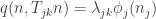
We consider a closed migration process on J colonies, with populations described by a vector $n=(n_1,\ldots,n_J)$ . We say that the instantaneous rate of movement of an individual from colony j to colony k is $q(n,T_{jk}n)=\lambda_{jk}\phi_j(n_j)$ , for some functions $\phi_j(0)=0$ . We can describe the ED of this system in terms of the distribution obtained when a single individual performs a random walk through the state space, with $\phi_j(1)$ taken to be 1 for each j. We call the DBEs for this case the traffic equations, with solutions $(\alpha_j,j\in J)$ . Then, by checking the PBEs, it is clear that the equilibrium distribution of the original migration process satisfies

$\pi(n)\propto \prod_{j=1}^J \frac{\alpha_j^{n_j}}{\prod_{r=1}^{n_j}\phi_j(r)}$

This is important, as it would have been computationally difficult to solve the original equations for an ED.

The same result holds for an open migration process, where individuals can enter and leave the system, arriving at colony j at rate $\nu_j$ , and leaving at rate $\mu_k\phi_k(n_k)$ . Note that this has the same form as if each colony was served by a PP( $\alpha_j\lambda_j$ ), with departures at rate $\lambda_j\phi_j(n_j):=(\mu_j+\sum_k\lambda_{jk})\phi_j(n_j)$ . But (obviously) this interpretation is not equivalent to the model

The time reversal is also an OMP. One has to check that the transition rates have the correct form, and so the exit process from each colony (in equilibrium, naturally), is PP( $\alpha_j\mu_j$ )$. Most importantly, given a communicating class, we can think of the restriction to this class as an OMP, so in particular, rates of transition between classes are Poisson.

Little’s Law

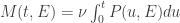
Informally, the mean number of customers should be equal to the arrival rate multiplied by the mean sojourn time in the system of a customer. This is easiest to formalise by taking an expectation up to a regeneration time. This is T, the first time the system returns to its original state (assumed to be 0 customers), an a.s. finite stopping time.

Set $L:=\mathbb{E}\frac{1}{T}\int_0^Tn(s)ds$ , the average number of customers, and $W:=\frac{\mathbb{E}\sum_1^N W_n}{\mathbb{E}N}$ where N is the number of customers arriving in [0,T], and $W_n$ is the waiting time of the n-th customer.

Little’s Law asserts that $L=\lambda W$ . Note that for a Markov Chain in equilibrium, can define L more simply as $\mathbb{E}n$ and similarly for W.

It is easiest proved by considering the area between the arrivals process and the departure process in two ways: integrating over height and width. Note that working up to a regeneration time is convenient because at that time the processes are equal.

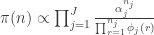
The migration processes above are said to be linear if $\phi_j(n_j)=n_j$ . This process has the form of a Markov chain, and so even in a more general state space, the distribution of points in disjoint subsets of the state-space are independent Poisson processes.

Often though, we start with no individuals in the system, but still the distribution is given by a time-inhomogenous Poisson random measure. The mean is specified by

$M(t,E)=\nu\int_0^t P(u,E)du$

where $\nu$ is the net arrival rate, and $P(u,E)$ is the probability that an individual is in E, a time interval of u after arriving.

As one would suspect, this is easiest to check through generating functions, since independence has a straightforward generating function analogue, and the expression for a Poisson RV is manageable.

One queue or many queues? (eventuallyalmosteverywhere.wordpress.com)

1 thought on “Queues and Migration Processes”

Pingback: Loss Networks and Erlang’s Fixed Point | Eventually Almost Everywhere

Eventually Almost Everywhere

A blog about probability and olympiads by Dominic Yeo

Queues and Migration Processes

1 thought on “Queues and Migration Processes”

Leave a Reply Cancel reply

Related articles

Share this:

Like this:

Related

1 thought on “Queues and Migration Processes”

Leave a Reply Cancel reply