Yesterday I introduced the notion of duality for two stochastic processes. My two goals for this post are to elaborate on the idea of why duality is useful, which we touched on in passing in the previous part, and to discuss duality of interacting particle systems. In the latter case, there are often nice ways to consider the forward and backward processes together that make the relation somewhat more natural.
The starting point is to assume a finite state space. This will be reasonable when we start to consider interacting particle systems, eg on ![\{0,1\}^{[n]}](https://s0.wp.com/latex.php?latex=%5C%7B0%2C1%5C%7D%5E%7B%5Bn%5D%7D&bg=ffffff&fg=333333&s=0&c=20201002) . As before, call the spaces R and S, and a duality function H(x,y). Since the state-spaces are finite, it is entirely natural to think of this as a matrix, and hence as an operator. Of course, a function defined on a finite state-space can be thought of as a vector, so it is clear what this operator will actually operate on. (I’ve chosen H rather than h for the duality function so it is more clear that it is acting as an operator here.)
. As before, call the spaces R and S, and a duality function H(x,y). Since the state-spaces are finite, it is entirely natural to think of this as a matrix, and hence as an operator. Of course, a function defined on a finite state-space can be thought of as a vector, so it is clear what this operator will actually operate on. (I’ve chosen H rather than h for the duality function so it is more clear that it is acting as an operator here.)
We have some choice about which way round to define it, but for now let’s say that given some function f(.) on S
Note that this is a) exactly the definition of matrix (left-)multiplication; b) We should think of Hf as a function on R – perhaps (Hf)(x) might be more clear? and c) the operator H acts  . If we want the corresponding operator
  , we simply multiply by H on the right instead.
But note also that the generator of a finite state-space Markov process is also a matrix, indeed a Q-matrix. So if we take our definition of the duality function as
which, importantly, holds for all x,y, we can convert this into an algebraic form as

In the same way that n-step transition probabilities for a discrete-time Markov chain are given by the product of the one-step transition matrix, general time transition probabilities for a continuous-time Markov chain are given by exponents of the Q-matrix. In particular, if X and Y have transition kernels P and Q respectively, then  , and after doing some manipulation, we can show that

also. This is really useful as in general we would hope that H might be invertible, from which we derive
So this is a powerful statement about the relationship between the evolutions of the two processes. In particular, it shows a correspondence (given by H) between left eigenvectors of P, and right eigenvectors of Q, and vice versa naturally.
The reason why this is useful rather than merely cute, is that when we re-interpret everything in terms of the original stochastic processes, we get a map between stationary distributions of X, and harmonic functions of Y. Stationary distributions are often hard to describe in any terms other than the left-1-eigenvector, or through some convergence property that is typically hard to work with. Harmonic functions, on the other hard, can be much more tractable. An example of a harmonic function is the survival probability started from a given state. This is useful for specifying the stationary distribution, but perhaps even more so for describing properties of the set of stationary distributions. In particular, uniqueness and existence are carried across this equivalence. So, for example, if the dual does not survive almost surely, then this says the only stationary measure is zero, and so the process is transient or similar.
Jan Swart’s course in Luminy last October dealt with duality, with a focus mainly on interacting particle systems. There are a couple of themes I want to talk about, without going into too much detail.
A typical interacting particle system will take place on a locally finite graph. At each vertex, there is either a particle, or there isn’t. Particles move between adjacent vertices, and sometimes interact with particles at adjacent vertices. These interactions might involve branching or coalescence. We will discuss shortly the set of possible forms such interaction might take. The state space is  , with G the underlying graph. Then given a state, there is some set of actions which might happen next, and we consider the possibility that they happen with exponential rates.
At this stage, it seems like the initial configuration is important, as this affects what set of moves can happen immediately, and also thereafter. It is not clear how quickly this dependence fades. One useful idea is not to restrict ourselves to interactions involving the particles currently present in the system, but instead to consider a Poisson process of all possible interactions. Only the moves actually permitted by the current state will happen, but having this extra information allows for coupling between initial configurations.
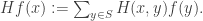
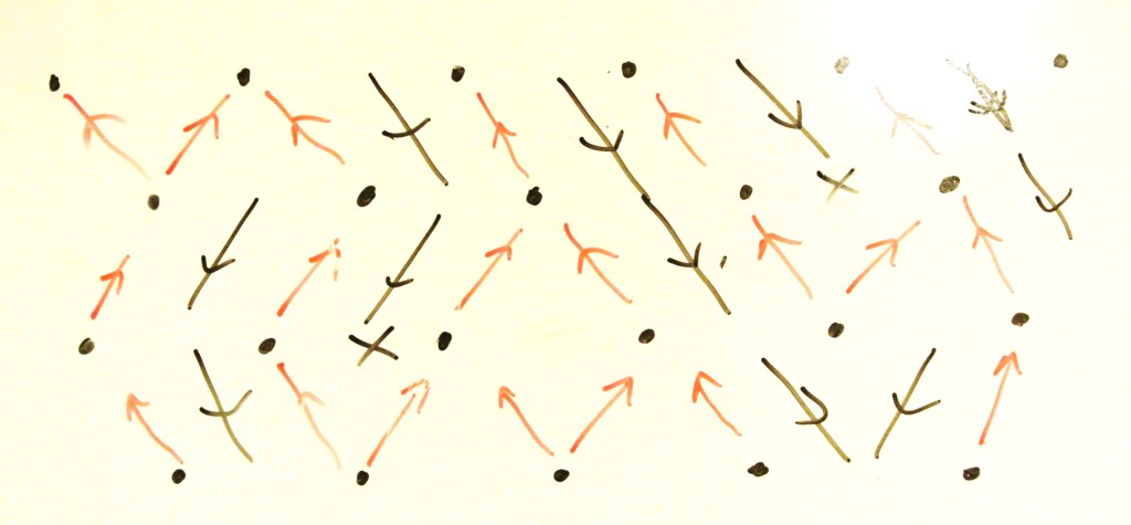
It’s probably easier to consider a concrete example. The picture below shows the set-up for a branching random walk up an integer lattice. Each particle moves to one of the two state directly above its current state, or it branches and sends particles to both of them. In the diagram, we have glued arrows onto every state at every time, which tells us what to do if there is a particle there at each time. As a coupling, we can now think of the process as a deterministic walk through a random environment. The environment is given by some probability space, which in continuous time might have the appearance of a Poisson process on the set of ‘moves’, and the initial condition of the walk is up to us.
We can generalise this to a broader class of interacting particle systems. If we want all interactions to be between pairs of adjacent states, there are six possible things which could happen:
- Annihilation: two adjacent particles destroy each other. ( 11 -> 00 )
- Branching: one particle becomes two particles. ( 01 or 10 -> 11 )
- Coalescence: two particles merge. ( 11 -> 01 or 10 )
- Death: A particle is removed. ( 01 or 10 -> 00 )
- Exclusion: a particle moves. ( 01 -> 10 )
- Birth: a particle is created. ( 00 -> 01 or 10 )
For now we exclude the possibility of birth. Note that the way we have set this up involving two-site interactions excludes the possibility of a particle trying to move to an already-occupied site.
 Let us say that in process X the rates at which each of these events happen are a, b, c, d and e, taking advantage of the helpful choice of naming. There is some flexibility about whether the rates are the same between every pair of vertices of note. For this post we assume that they are. Then it is a result of Lloyd and Sudbury that given some real
  , the process X’ with corresponding rates given by:

for 
is dual to X, with duality function given by  , for Y and Z possible states.
I want to make two comments:
1) This illustrates one of the differences between the dual and the time-reversal. It is clear that the time-reversal of branching is coalescence and vice versa, and exclusion is invariant under time-reversal. But the time-reversal of death is definitely birth, but there is no birth component in the dual of a process which features death. I don’t have a strong intuition for why this is the case, but see the final paragraph of this post. However, at least it seems plausible that both processes might simultaneously be recurrent, since in the dual, both the branching rate and the death rate have increased by the same amount.
2) This settles one problem of uniqueness of the dual that I mentioned last time, since we can vary q and get a different dual to the same original process. For example, in the voter model, we have b=d=1, and a=c=e=0, as in any update, the opinions of neighbours which were previously different become the same. Anyway, for any ![q\in[-1,0]](https://s0.wp.com/latex.php?latex=q%5Cin%5B-1%2C0%5D&bg=ffffff&fg=333333&s=0&c=20201002) there is a choice of dual, where at the extremes q=0 corresponds to coalescing random walk, and q=-1 to annihilating random walk. (Note that the duality function for q=0 is the indicator function that the systems are different.)
there is a choice of dual, where at the extremes q=0 corresponds to coalescing random walk, and q=-1 to annihilating random walk. (Note that the duality function for q=0 is the indicator function that the systems are different.)

As a final observation without much justification, suppose we add in arrows in the gaps of the branching random walk picture we had earlier, and direct them in the opposite direction. It turns out that this corresponds precisely to the dual of the process. This provides an appealing visual idea of why the dual of branching might be death. It also supports the general idea based on the coupling described earlier that the dual process is in some sense a deterministic walk in the opposite direction through the random environment specified by the original process.
REFERENCES
J.M. Swart – Duality and Intertwining of Markov Chains (mainly using chapters 2.1 and 2.7)
Thanks for Daniel Straulino for direction towards the branching random walk duality example.


vertices have type i.
(for
) is present, independently, with probability
have type 1,
have type 2, etc etc. This makes no difference except in terms of the notation we have to use if we want to use exchangeability arguments later.
on [k], and assigns the types of the vertices of [n] in an IID fashion according to
. The exponential form has a more natural interpretation if we ever need to turn the IRGs into a process. Additionally, it avoids the requirement to treat small values of n (for which, a priori,
might be greater than 1) separately.


![\pi=(\pi_1,\ldots,\pi_k)\in[0,1]^k](https://s0.wp.com/latex.php?latex=%5Cpi%3D%28%5Cpi_1%2C%5Cldots%2C%5Cpi_k%29%5Cin%5B0%2C1%5D%5Ek&bg=ffffff&fg=333333&s=0&c=20201002)


, the number of type j neighbours of
.
.
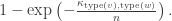
![p_j\left[1-\exp\left(-\frac{\kappa_{i,j}}{n}\right)\right]\approx \frac{p_j\cdot \kappa_{i,j}}{n} \approx \kappa_{i,j}\pi_j](https://s0.wp.com/latex.php?latex=p_j%5Cleft%5B1-%5Cexp%5Cleft%28-%5Cfrac%7B%5Ckappa_%7Bi%2Cj%7D%7D%7Bn%7D%5Cright%29%5Cright%5D%5Capprox+%5Cfrac%7Bp_j%5Ccdot+%5Ckappa_%7Bi%2Cj%7D%7D%7Bn%7D+%5Capprox+%5Ckappa_%7Bi%2Cj%7D%5Cpi_j&bg=ffffff&fg=333333&s=0&c=20201002)
 , since it’s easy to do vector and matrix calculations when most of the entries of all the vectors are zero. We also have a good visual idea (at least in up to three dimensions) of what a matrix might mean with respect to that basis. If we needed to divide the three-dimensional world around us into small volumes, we’d tend to describe it with small cubes rather than small arbitrary parallelopipeds.
 , where D is a diagonal matrix. We construct P by taking its columns to be these eigenvectors. In particular, for a given vector x, y=Px is the vector giving the coefficients of x in the basis of eigenvectors.
 , then x is in the kernel of
  . As we discussed last time, introducing the determinant gives a much more manageable way to verify which values of
  result in
  , and this leads to a polynomial of degree n (the dimensional of the vector space / size of the matrix) for
  , which has the eigenvalues as its roots.
 for example has no fixed vectors.
 of an eigenvalue
  in the factorisation of the characteristic polynomial. To define the geometric multiplicity, observe that all the eigenvectors with eigenvalue
  . There are two facts that one needs to remember. The slightly less obvious one is that
  for all
 , where the 2s can be replaced by any value, and the 1 can be replaced by an non-zero value. There’s plenty to learn about to what extent versions of this matrix of higher size represent all non-diagonalisable matrices, but such an exposition of Jordan normal form comes next year for the students taking this course.
 and ending up at our counter-example. One could also argue from this that the set of non-diagonalisable matrices are dense within the set of matrices with a repeated eigenvalue. That is, having a repeated eigenvalue but full eigenspace is doubly-infinitely-unlikely.
 , where the zero on the right-hand side is the zero matrix. It’s tempting to substitute A into the expression
  , but of course this is not valid. Indeed imagine a typical eigenvalue determinant matrix with terms like
  on the diagonal; it doesn’t make sense to substitute a matrix for
  is a matrix. Now looki at the action of
 for all v, hence
  is a monic polynomial, all of whose non-leading coefficients are multinomials of degree at most n-1 in the entries of A. Furthermore, these multinomials have (non-negative) integer coefficients. Therefore the entries of
  ) the function
  , the multiset of roots is continuous in the coefficients of the polynomial.
 be the characteristic polynomial of A. Each
  is a polynomial of degree
  in the entries of A. Let’s consider now a matrix-valued function A(t), and we assume that the entries of A(t) are all differentiable with respect to t. So each
  is also differentiable with respect to t.
 be some eigenvalue of A(t), chosen such that
  , the eigenvalue with largest absolute value (with some canonical tie-breaking mechanism). Then
  , and so differentiating with respect to
 , and so
 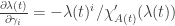 . In particular,
  such that
  has a repeated eigenvalue. Then, in a small enough region of
  continuously such that
  while
while  for
for  . Then, if the entries of A(t) are analytic functions of t, then so are
  will in general not be analytic, as the maximum of two smooth functions is in general Lipschitz.
 , for which the largest eigenvalue is
  .
. with
with  , we have
 should have direction close to that of the eigenvector, for any test vector v. The rate of convergence depends on the ratio of the largest eigenvalue to the second largest eigenvalue, though if the matrix is not diagonalisable, it is not completely trivial to quantify this convergence. We have to be careful though, since A maps the subspace orthogonal to the eigenvector to itself, so the magnitude of the projection of v onto the eigenvector determines the speed of convergence. Indeed, if v is orthogonal to the eigenvector, it won’t converge towards the principal eigenvector at all. (But if there is a well-defined ‘second eigenvector’ then it will converge towards that.)
 is an eigenvector of matrix A with eigenvalue
  (*)
(*) . So given a matrix
  with eigenvalue
  corresponding to eigenvector
  , in a neighbourhood of
  we can use the implicit function theorem to comment on the differentiability of
 are (1,0) and (0,1), while the eigenvectors of
  are (1,1), (1,-1). So no continuous choice of eigenvectors is possible here.
 . This is good, as otherwise we would be free to replace any norm by an arbitrary multiple of itself, and so no useful bounds could ever emerge. Note that the submultiplicativity implies that
  .
. be some eigenvalue and associated (right-)eigenvector respectively of matrix A. Let X be the square matrix given by taking all the columns to be x. Now
  , and so
 .
.
 , we derive Gelfand’s Formula, that
  . Again, this applies for any matrix norm.
 , then for any
  , and equality is attained when x is the respective eigenvector, normalised appropriately.
 is a convex function of the (real, symmetric) matrix.
 , arrange them in an nxk matrix P, so that
  . Now we consider the matrix
  . [Note that if k=1, we are exactly considering
  as before.] Then Poincare’s Separation Theorem say that the eigenvalues
  of
of 
 . Without loss of generality, we may assume the basis has been chosen so that the diagonal elements of A satisfy
  , and so now we have that the sequence
  is majorised by
  and majorises
  . The first of these relations can be used via the setup of Karamata’s inequality to conclude that for any convex function f, we have

 , and take absolute values and apply the triangle inequality,
 to be the sum of the non-diagonal entries of the ith row. Then the Gershgorin circle theorem says that every eigenvalue lies within at least one of the discs
  , in the complex plane. So our motivation still makes sense. If the off-diagonal entries are small, this is a strong restriction, and if they are not typically smaller than the diagonal entries, then we perhaps do not learn very much. Obviously, we could apply the same argument to the columns too.
![z\in[0,1]](https://s0.wp.com/latex.php?latex=z%5Cin%5B0%2C1%5D&bg=ffffff&fg=333333&s=0&c=20201002) and observe what happens as z varies from 0 to 1. When z=0, the matrix is diagonal, and each eigenvalue is in the Gershgorin disc (which is a single complex number). As z varies continuously, the characteristic polynomial varies continuously, and also its roots, that is the set of eigenvalues. So since each of the r eigenvalues are initially within the union of the r original, large Gershgorin discs, they must remain within this union as z varies, since they cannot ‘jump’ to another component.
and observe what happens as z varies from 0 to 1. When z=0, the matrix is diagonal, and each eigenvalue is in the Gershgorin disc (which is a single complex number). As z varies continuously, the characteristic polynomial varies continuously, and also its roots, that is the set of eigenvalues. So since each of the r eigenvalues are initially within the union of the r original, large Gershgorin discs, they must remain within this union as z varies, since they cannot ‘jump’ to another component.


 . If we consider the distribution of
  , this is given by
  , where
  . Note it is not immediately equivalent to saying that P has a stationary distribution, as the latter must be non-negative and have elements summing to one. Only the first property is difficult, and relies on some
  , and in general, there will be a single eigenvalue (ie dimension 1 eigenspace) with
  , and the rest satisfies
  . Then, if we diagonalise P, it is clear why
  converges entry-wise, as
  converges. In the latter, only the entries in the row corresponding to
  converge to something non-zero.
 , provided we two conditions hold. The conditions are that the chain is irreducible and aperiodic.
 and
and  , so any affine combination of the two
  will give a stationary distribution for the whole chain.
 for
for  a closed communicating class, then we know that
  whenever
  . For the remaining j, we can use the theorem in its original form on the Markov chain, with state space reduced to A. Here, it is now irreducible.
 . Then, we decompose this large number of steps so to say that not only have we entered A with roughly the given probability, but in fact with roughly the given probability we entered A a long time in the past, and so there has been enough time for the original convergence result to hold in A.
 , such that
  . Equivalently, the directed graph describing the possible transitions of the chain is k-partite. This definition makes it immediately clear that
  will converge. Indeed, to verify this, we would need to consider the Markov chain with transition matrix
  . Note that this is no longer irreducible, as it there are no transitions allowed between classes
  s satisfies the conditions of the theorem.
 , let’s assume A has size 2 and period 2. That is, once we arrive in A, thereafter we alternate deterministically between the two states. Anyway, for some large time n, we can write
  for
for  as:
as:


 (1)
(1) is a right- or column eigenvector of P, with eigenvalue 1. Since the spectrum of
  is the same as that of P, we conclude that 1 is a left-eigenvalue of P also. So we can be assured of the existence of a vector
  , it is possible to move from i to j and back again. In terms of the transition matrix, P is irreducible if it is not block upper-triangular, up to reordering rows and columns.
 satisfies (1).
 and
and  , and it is not hard to see that for any eigenvector with negative and non-negative components, the sign of a component is a class property.
 stochastic matrix P, and a 1-eigenvector
  are first. That is, in a moderate abuse of notation:
 and
and  are both zero. This implies that states in A and states in B do not communicate, showing that P is reducible. We can formulate this as a linear programming problem:
 , and assume that
  , that is, there are a positive number of negative and non-negative components. Noting that the sum of the rows in a stochastic matrix is 1, we may consider instead:


 , then we say it is an invariant distribution. Of course, if I is finite, then any invariant measure can be normalised to give an invariant distribution.
 is transient, but the uniform measure is invariant. However, it is not a sufficient condition for the existence of an invariant distribution either. (Of course, an irreducible finite chain is always recurrent, and always has an invariant distribution, so now we are considering only the infinite state space case.) The random walk on
  is recurrent, but the invariant measure is not normalisable.
 , where
  is the the return time starting from some
  .
. are all equal in distribution. Note that the dependence structure remains complicated, and much much more interesting than the individual distributions. Next, we observe that a calculation of n-step transition probabilities for a finite chain will typically involve a linear combination of nth powers of eigenvalues. One of the eigenvalues is 1, and the others lie strictly between -1 and 1. We observe in examples that the constant coefficient in
  , some distribution on I. By considering
  , it is easy to see that if this converges,
  is an invariant distribution. The classic examples which do not work are
 and
and  ,
, is a function of the remainder of n modulo 3 alone. With a little thought, we can give a precise classification of such chains which force you to be in particular proper subsets of the state space at regular times n. Chains without this property are called aperiodic, and we can show that distributions for such chains converge to the equilibrium distribution as