After the general discussion of Levy processes in the previous post, we now discuss a particular class of such processes. The majority of content and notation below is taken from chapters 1-3 of Jean Bertoin’s Saint-Flour notes.
We say 
- It is a right-continuous adapted stochastic process, started from 0.
- It has stationary, independent increments.
- It is increasing.
Note that the first two conditions are precisely those required for a Levy process. We could also allow the process to take the value 
Examples
- A compound Poisson process, with finite jump measure supported on
. Hereafter we exclude this case, as it is better dealt with in other languages.
- A so-called stable Levy process, where
, for some
. (I’ll define
very soon.) Note that checking that the sample paths are increasing requires only that
almost surely.
- The hitting time process for Brownian Motion. Note that this does indeed have jumps as we would need. (This has
.)
Properties
- In general, we describe Levy processes by their characteristic exponent. As a subordinator takes values in

- We can refine the Levy-Khintchine formula;

- where k is the kill rate (in the non-strict case). Because the process is increasing, it must have bounded variation, and so the quadratic part vanishes, and we have a stronger condition on the Levy measure:
.
- The expression
for the tail of the Levy measure is often more useful in this setting.
- We can think of this decomposition as the sum of a drift, and a PPP with characteristic measure
. As we said above, we do not want to consider the case that X is a step process, so either d>0 or
is enough to ensure this.
Analytic Methods
We give a snapshot of a couple of observations which make these nice to work with. Define the renewal measure U(dx) by:

If we want to know the distribution function of this U, it will suffice to consider the indicator function 
The reason to exclude step processes specifically is to ensure that X has a continuous inverse:


In fact, this renewal measure characterises the subordinator uniquely, as we see by taking the Laplace transform:


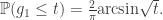
The Arcsine Law
X is Markov, which induces a so-called regenerative property on the range of X, 


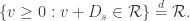
In fact, the converse holds as well. Any random set with this regenerative property is the range of some subordinator. Note that 
In particular, we consider the last passage time 


The most natural application of this is to the hitting time process of Brownian Motion, which is stable with 


So