Trap models and laws of not-so-large numbers

Posted on August 4, 2017 by dominicyeo

I’m back in Rio, this time for the Brazilian Probability School, which this year is being held in parallel with the Brazilian Mathematical Colloquium, so there’s a lot of possible lectures to be attending across a wide range of topics. I’ve been paying particular to a course by Veronique Gayrard concerning the phenomenon of aging, as seen in various spin-glass and trap models. [Lecture notes exist, but haven’t yet been put online.]

I want to write something about the setup for one of these models. It took me quite a long time to settle on a title for this post, and as you can see I’ve hedged. At least in this post, I’m not so interested in the model (and don’t want to try and offer a physical motivation at this point) but rather in talking about the natural model-independent problem it reduces to.

Motivation

Let $X_1,X_2,X_3,\ldots$ be IID random variables which take some fixed value K>0 with probability 1/K, and otherwise take the value zero. The law of large numbers says that for large m, the rescaled partial sum process $\frac{1}{m}(X_1+\ldots+X_m) \approx 1$ . The weak LLN makes this precise in the sense of convergence in distribution, and the strong LLN gives almost sure convergence.

But the speed of convergence is obviously not uniform over all distributions of the underlying IID random variables. This is particularly clear in the setup I’ve outlined, in the regime where $K\rightarrow\infty$ . Certainly if $1\ll m\ll K$ , then we have $\frac{1}{m}(X_1+\ldots+X_m) \ge \frac{K}{m}$ with probability $\approx \frac{m}{K}$ and otherwise $\frac{1}{m}(X_1+\ldots+X_m) = 0$ . So if we let K and m diverge together with scaling as given, the only version of a LLN we can write down is

$\frac{1}{m}(X_1+\ldots+X_m)\stackrel{d}\rightarrow 0,$

which is obviously different to the original version for fixed K and diverging m.

If we take $m=\Theta(K)$ , then the rescaled partial sum process converges in distribution to a scaled Poisson process. Of course, the Poisson process obeys it’s own law of large numbers (or law of large times), but on this scale the first-order behaviour is random.

At a more general level, what we are doing in the previous examples is looking at a process which converges to equilibrium, but studying it on a faster timescale than the timescale of this convergence. The REM-like trap model, which will be the eventual focus of this post, does exactly this to a continuous-time Markov chain, with the additional factor that the holding rates are random and heavy-tailed.

The mean-field REM-like trap model

This REM-like trap model is defined as follows. We have N sites, and for these sites we sample an IID collection of holding rates $(\tau_N(1),\ldots,\tau_N(N))$ according to some distribution. We then choose a sequence of a IID uniform samples from {1,…,N}, labelled $(J_N(1),J_N(2),\ldots)$ . We think of this as recording an itinerary of visits to the sites, where the jth site we visit is $J_N(j)$ . (Though notice that under this definition, it’s possible that the jth site we visit and the j+1st site we visit are the same.) We wait at each site for an exponential holding time, with parameter $\tau_N(j)$ if we are at site j, and these holding times are independent of the other holding times, and independent of the trajectory, all conditional on $(\tau_N(1),\ldots,\tau_N(N))$ .

You can think of this as a continuous-time RW on the complete graph $K_N$ (with self-loops), where the jump chain is uniform, and the holding rates are given by $(\tau_N(1),\ldots,\tau_N(N))$ . This explains the notation, and how you’d construct a similar model on a different underlying graph.

The general of a trap model is a random walk with very inhomogeneous speed, for example because some holding times have very large expectation. In a setting with more inbuilt geometry, for example on a lattice, we can imagine the RW getting trapped in regions associated with atypically low speeds. We might therefore think of a site with very long holding times as being deep, in the sense that the chain might get stuck there.

This will be most interesting if we allow an extreme range of values taken by $\tau_N$ , and so the best choice is a distribution in the domain of attraction of an $\alpha$ -stable law with parameter $\alpha\in(0,1)$ . That is $\mathbb{P}(\tau \ge u) = u^{-\alpha}L(u)$ , where L is a slowly-varying function at $+\infty$ .

This distribution has infinite mean, and so we couldn’t apply either LLN to a sequence of copies of $\tau$ . However, obviously the sequence $(\tau_N(1),\ldots,\tau_N(N))$ almost surely does have finite mean, since each entry is finite! So for each N, the trap model will have a LLN on large timescales, but we will investigate at faster timescales.

The clock process

At least for the purpose of this post, we will focus on the clock process, which records the (continuous) time which elapses before we arrive at the *k*th state of the jump chain.

That is,

$S_N(0)=0, \quad S_N(k) = \sum_{i=0}^k \mathrm{Exp}\left(1/\tau_N(J_N(i))\right),$

where the exponential random variables are independent except through their parameters. This can be made even more clear if we take advantage of the method to write a general exponential distribution as a multiple of a exponential distribution with parameter 1. Let $e_0,e_1,\ldots$ be IID exponential RVs independent of $(\tau_N(1),\ldots,\tau_N(N))$ and the jump chain. Then

$S_N(k)=\sum_{i=0}^k \tau_N(J_N(i)) e_i.$

Let’s briefly pause to apply the LLN to $S_N$ for fixed N. It matters whether we consider the quenched or annealed settings here. As usual, quenched means we fix a realisation of the random environment, and draw all conclusions in terms of that environment (think of conditional expectations). And annealed means that we also include the randomness of the environment. This is notationally annoying, so as a shorthand we write $\mathbb{E}_{\tau_N}$ for quenched expectations $\mathbb{E}[\cdot \,|\, \tau_N(1),\ldots,\tau_N(N)]$ , and $\mathbb{E}$ for an expectation over all randomness.

Then the quenched rate of growth of $S_N$ is given by

$\mathbb{E}_{\tau_N}\left[ \frac{S_N(k)}{k}\right] = \frac{\tau_N(1)+\ldots +\tau_N(N)}{N},$

and so the annealed rate

$\mathbb{E}\left[\frac{S_N(k)}{k}\right] = \infty,$

since $\mathbb{E}[\tau_N(1)]=\infty$ . But as in the introduction, these rates are only relevant to laws of large numbers when k grows on a large enough timescale, and we will consider smaller scales of k.

Timescales of the clock process

We’re going to look for scaling limits of the clock process. The increments are ‘sort of IID’ and ‘sort of heavy-tailed’ (we’ll clarify these sort ofs when we need to) so it wouldn’t be surprising if the scaling limits are Levy processes. The clock process is increasing, so in fact the scaling limits should be subordinators, and it wouldn’t be surprising if under some circumstances they turned out to be stable subordinators.

There is flexibility about how to do the rescaling. From now on, we are working in a $N\rightarrow\infty$ regime. Let’s assume we look at $t a_N$ steps of the jump chain, where $(a_N)$ is some divergent sequence. A property of large sums of IID stable distributions with parameter $\alpha\in(0,1)$ is that the scaling of the value of the sum is comparable to the scale of the largest summand. That is, the partial sum is dominated by its largest summands. Compare with the standard case for non-negative RVs, where for k summands, the sum is $\Theta(k)$ , while the largest summand is $O(\log k)$ .

So to identify the scale of the clock process after $a_N$ steps of the jump chain, it’s sufficient to identify the scale of its expected largest holding time. All of this is vague at the level of constants, so we choose a divergent sequence $(c_N)$ for which

$\mathbb{P}(\tau_N(1) \ge c_N) = \Theta\left(\frac{1}{a_N}\right).$

Note 1: this means that the number of holding times among the first $a_N$ which are at least $c_N$ is binomial with $\Theta(1)$ expectation. The fact that is well-approximated by a Poisson distribution will be relevant shortly.

Note 2: because we already insisted that $\tau(x)$ had a slowly-varying tail, this gives control of the $\mathbb{P}(\tau_N(1)\ge 5c_N)$ etc as well.

We expect that $S_N(t a_N) = \Theta(c_N)$ , and so we consider scaling limits of the process

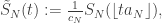
$\tilde S_N(t):= \frac{1}{c_N} S_N(\lfloor t a_N \rfloor),$

as usual. [Note I am using the opposite convention to VG’s notes, where ~ denotes the unrescaled clock process.]

Scaling limits

We identify two types of scaling limit, depending on whether $a_N\ll N$ or $a_N = \Theta(N)$ . The former is called an intermediate timescale, while the latter is an extreme timescale. After this long motivation and notational preliminary section, my goal is to explain (partly to myself) why these scaling limits are different.

First, we state the result for intermediate timescales. Let $S^{\mathrm{int}}$ be the stable subordinator with parameter $\alpha$ , that is with Levy measure $\alpha \Gamma(\alpha)u^{-\alpha}$ . Then $\tilde S_N \Rightarrow S^{\mathrm{int}}$ , in the Skorohod topology. We need to be clear about the sense of convergence, and the role of the random environment. It turns out that if in addition $a_N\ll \frac{N}{\log N}$ , then this convergence holds for almost all realisations of the random environment. That is, the laws of the processes (with respect to the randomness of the jump chain / holding times etc) converge. When $a_N$ is only $\ll N$ , then the convergence holds in probability with respect to the environment. It took me a while to parse what this means. It means that for large N, the probability that the random environment induces a law of $\tilde S_N$ which is far from the law of $S^{\mathrm{int}}$ tends to zero.

The exact Levy triple of the limit process is not the important message here, and if that’s unfamiliar, then it isn’t a problem. The point is that you would also get this limiting Levy process if you took the sum process of genuinely IID random variables with the same $\alpha$ -tail. And this is not surprising. Since recall that in the intermediate timescale $a_N\ll N$ , so during the first $t a_N$ steps of the jump chain, we do not typically visit many sites more than once. Indeed, if $a_N\ll \sqrt{N}$ , then this is the birthday problem, and we typically visit no site more than once. However, even in the weaker setting $a_N\ll N$ , look at the deepest 1000 sites we visit during the first $ta_N$ steps. We can compute that, in expectation, we visit essentially zero of these more than once. But these 1000 sites dominate the clock process at $ta_N$ . So from the point of view of the clock process, since we hardly ever visit relevant sites twice, the depths $\tau_N(J_N(1)),\tau_N(J_N(2)),\ldots$ are essentially independent, and so it’s unsurprising that we get the scaling limit corresponding to IID partial sums.

For extreme timescales, by contrast, this fails. If we take $a_N=1000 N$ , we expect to visit each site roughly 1000 times, indeed the number of visits to a given site will be approximately $\mathrm{Poisson}(1000)$ . But it’s still the case that the scaling limit will be dominated by the deepest sites. In particular, at some point on this timescale we will visit the deepest site, and indeed we will visit it multiple times if we look at $ta_N$ for large t. So the jumps of any scaling limit are not independent any more unless we condition on all the depths $\tau_N$ .

However, all is not lost, since we can show that the point process of rescaled depths $\sum \delta_{\tau_N(i)/c_N}$ converges to a Poisson random measure on $[0,\infty)$ . The candidate for the scaling limit of the clock process is then the subordinator whose Levy measure is this Poisson random measure. This isn’t itself a Levy process, but it is a mixture of Levy processes, reflecting that on extreme timescales the quenched and annealed viewpoints are different since there is enough time to visit the whole landscape.

Heuristically, the extreme timescale is the entry point for convergence to equilibrium. Indeed, taking $t\rightarrow\infty$ , the number of visits to each of the 1000 top sites converge to their expectation, corresponding to convergence of the clock process to equilibrium, since these holding times continue to dominate the sum. The clock process therefore starts to feel the finiteness of the state space, which introduces dependence between the most relevant holding times, which was not the close on intermediate timescales.

In the next post, I’m going to try and summarise VG’s descriptions of taking this model beyond the mean-field setting, where the range of possibilities becomes much much richer. I’m also going to try and say something and glassy dynamics and ageing, and why the physical motivation justifies considering these particular models and scalings.

Subordinators and the Arcsine rule

Posted on December 5, 2012 by dominicyeo

After the general discussion of Levy processes in the previous post, we now discuss a particular class of such processes. The majority of content and notation below is taken from chapters 1-3 of Jean Bertoin’s Saint-Flour notes.

We say $X_t$ is a subordinator if:

It is a right-continuous adapted stochastic process, started from 0.
It has stationary, independent increments.
It is increasing.

Note that the first two conditions are precisely those required for a Levy process. We could also allow the process to take the value $\infty$ , where the hitting time of infinity represents ‘killing’ the subordinator in some sense. If this hitting time is almost surely infinite, we say it is a strict subordinator. There is little to be gained right now from considering anything other than strict subordinators.

Examples

A compound Poisson process, with finite jump measure supported on $[0,\infty)$ . Hereafter we exclude this case, as it is better dealt with in other languages.
A so-called stable Levy process, where $\Phi(\lambda)=\lambda^\alpha$ , for some $\alpha\in(0,1)$ . (I’ll define $\Phi$ very soon.) Note that checking that the sample paths are increasing requires only that $X_1\geq 0$ almost surely.
The hitting time process for Brownian Motion. Note that this does indeed have jumps as we would need. (This has $\Phi(\lambda)=\sqrt{2\lambda}$ .)

Properties

In general, we describe Levy processes by their characteristic exponent. As a subordinator takes values in $[0,\infty)$ , we can use the Laplace exponent instead:

$\mathbb{E}\exp(-\lambda X_t)=:\exp(-t\Phi(\lambda)).$

We can refine the Levy-Khintchine formula;

$\Phi(\lambda)=k+d\lambda+\int_{[0,\infty)}(1-e^{-\lambda x})\Pi(dx),$

where k is the kill rate (in the non-strict case). Because the process is increasing, it must have bounded variation, and so the quadratic part vanishes, and we have a stronger condition on the Levy measure: $\int(1\wedge x)\Pi(dx)<\infty$ .
The expression $\bar{\Pi}(x):=k+\Pi((x,\infty))$ for the tail of the Levy measure is often more useful in this setting.
We can think of this decomposition as the sum of a drift, and a PPP with characteristic measure $\Pi+k\delta_\infty$ . As we said above, we do not want to consider the case that X is a step process, so either d>0 or $\Pi((0,\infty))=\infty$ is enough to ensure this.

Analytic Methods

We give a snapshot of a couple of observations which make these nice to work with. Define the renewal measure U(dx) by:

$\int_{[0,\infty)}f(x)U(dx)=\mathbb{E}\left(\int_0^\infty f(X_t)dt\right).$

If we want to know the distribution function of this U, it will suffice to consider the indicator function $f(x)=1_{X_t\leq x}$ in the above.

The reason to exclude step processes specifically is to ensure that X has a continuous inverse:

$L_x=\sup\{t\geq 0:X_t\leq x\}$ so $U(x)=\mathbb{E}L_x$ is continuous.

In fact, this renewal measure characterises the subordinator uniquely, as we see by taking the Laplace transform:

$\mathcal{L}U(\lambda)=\int_{[0,\infty)}e^{-\lambda x}U(dx)=\mathbb{E}\int e^{-\lambda X_t}dt$

$=\int \mathbb{E}e^{-\lambda X_t}dt=\int\exp(-t\Phi(\lambda))dt=\frac{1}{\Phi(\lambda)}.$

The Arcsine Law

X is Markov, which induces a so-called regenerative property on the range of X, $\mathcal{R}$ . Formally, given s, we do not always have $s\in\mathcal{R}$ (as the process might jump over s), but we can define $D_s=\inf\{t>s:t\in\mathcal{R}\}$ . Then

$\{v\geq 0:v+D_s\in\mathcal{R}\}\stackrel{d}{=}\mathcal{R}.$

In fact, the converse holds as well. Any random set with this regenerative property is the range of some subordinator. Note that $D_s$ is some kind of dual to X, since it is increasing, and the regenerative property induces some Markovian properties.

In particular, we consider the last passage time $g_t=\sup\{s<t:s\in\mathcal{R}\}$ , in the case of a stable subordinator with $\Phi(\lambda)=\lambda^\alpha$ . Here, $\mathcal{R}$ is self-similar with scaling exponent $\alpha$ . The distribution of $\frac{g_t}{t}$ is thus independent of t. In this situation, we can derive the generalised arcsine rule for the distribution of $g_1$ :

$\mathbb{R}(g_1\in ds)=\frac{\sin \alpha\pi}{\pi}s^{\alpha-1}(1-s)^{-\alpha}ds.$

The most natural application of this is to the hitting time process of Brownian Motion, which is stable with $\alpha=\frac12$ . Then $g_1=S_1-B_1$ , in the usual notation for the supremum process. Furthermore, we have equality in distribution of the processes (see previous posts on excursion theory and the short aside which follows):

$(S_t-B_t)_{t\geq 0}\stackrel{d}{=}(|B_t|)_{t\geq 0}.$

So $g_1$ gives the time of the last zero of BM before time 1, and the arcsine law shows that its distribution is given by:

$\mathbb{P}(g_1\leq t)=\frac{2}{\pi}\text{arcsin}\sqrt{t}.$

The Levy-Khintchine Formula

Posted on December 4, 2012 by dominicyeo

Because of a string of coincidences involving my choice of courses for Part III and various lecturers’ choices about course content, I didn’t learn what a Levy process until a few weeks’ ago. Trying to get my head around the Levy-Khintchine formula took a little while, so the following is what I would have liked to have been able to find back then.

A Levy process is an adapted stochastic process started from 0 at time zero, and with stationary, independent increments. This is reminiscent, indeed a generalisation, of the definition of Brownian motion. In that case, we were able to give a concrete description of the distribution of $X_1$ . For a general Levy process, we have

$X_1=X_{1/n}+(X_{2/n}-X_{1/n})+\ldots+(X_1-X_{1-1/n}).$

So the distribution of $X_1$ is infinitely divisible, that is, can be expressed as the distribution of the sum n iid random variables for all n. Viewing this definition in terms of convolutions of distributions may be more helpful, especially as we will subsequently consider characteristic functions. If this is the first time you have seen this property, note that it is not a universal property. For example, it is not clear how to write a U[0,1] random variable as a convolution of two iid RVs. Note that exactly the same argument suffices to show that the distribution of $X_t$ is infinitely divisible.

It will be most convenient to work with the characteristic functions

$\mathbb{E}\exp(i\langle \lambda,X_t\rangle).$

By stationarity of increments, we can show that this is equal to

$\exp(-\Psi(\lambda)t)\quad\text{where}\quad \mathbb{E}\exp(i\langle \lambda,X_1\rangle)=:\exp(-\Psi(\lambda)).$

This function $\Psi(\lambda)$ is called the characteristic exponent. The argument resembles that used for Cauchy’s functional equations, by dealing first with the rationals using stationarity of increments, then lifting to the reals by the (right-)continuity of

$t\mapsto \mathbb{E}\exp(i\langle \lambda,X_t\rangle).$

As ever, $\Psi(\lambda)$ uniquely determines the distribution of $X_1$ , and so it also uniquely determines the distribution of Levy process. The only condition on $\Psi$ is that it be the characteristic function of an infinitely divisible distribution. This condition is given explicitly by the Levy-Khintchine formula.

Levy-Khintchine

$\Psi(\lambda)$ is the characteristic function of an infinitely divisible distribution iff

$\Psi(\lambda)=i\langle a,\lambda\rangle +\frac12 Q(\lambda)+\int_{\mathbb{R}^d}(1-e^{i\langle \lambda,x\rangle}+i\langle \lambda,x\rangle 1_{|x|<1})\Pi(dx).$

for $a\in\mathbb{R}^d$ , Q a quadratic form on $\mathbb{R}^d$ , and $\Pi$ a so-called Levy measure satisfying $\int (1\wedge |x|^2)\Pi(dx)<\infty$ .

This looks a bit arbitrary, so first let’s explain what each of these terms ‘means’.

$i\langle a,\lambda\rangle$ comes from a drift of $-a$ . Note that a deterministic linear function is a (not especially interesting) Levy process.
$\frac12Q(\lambda)$ comes from a Brownian part $\sqrt{Q}B_t$ .

The rest corresponds to the jump part of the process. Note that a Poisson process is an example of a Levy process, hence why we might consider thinking about jumps in the first place. The reason why there is an indicator function floating around is that we have to think about two regimes separately, namely large and small jumps. Jumps of size bounded below cannot happen too often as otherwise the process might explode off to infinity in finite time with positive probability. On the other hand, infinitesimally small jumps can happen very often (say on a dense set) so long as everything is controlled to prevent an explosion on the macroscopic scale.

There is no canonical choice for where the divide between these regimes happens, but conventionally this is taken to be at $|x|=1$ . The restriction on the Levy measure near 0 ensures that the sum of the squares all jumps up some finite time converges absolutely.

$\Pi\cdot 1_{|x|\geq 1}$ gives the intensity of a standard compound Poisson process. The jumps are well-spaced, and so it is a relatively simple calculation to see that the characteristic function is

$\int_{\mathbb{R}^d}(1-e^{i\langle \lambda,x\rangle})1_{|x|\geq 1}\Pi(dx).$

The intensity $\Pi\cdot 1_{|x|<1}$ gives infinitely many hits in finite time, so if the expectation of this measure is not 0, we explode immediately. We compensate by drifting away from this at rate

$\int_{\mathbb{R}^d}x1_{|x|<1}\Pi(dx).$

To make this more rigorous, we should really consider $1_{\epsilon<|x|<1}$ then take a limit, but this at least explains where all the terms come from. Linearity allows us to interchange integrals and inner products, to get the term

$\int_{\mathbb{R}^d}(1-e^{-i\langle \lambda,x\rangle}+i\langle\lambda,x\rangle 1_{|x|<1})\Pi(dx).$

If the process has bounded variation, then we must have Q=0, and also

$\int (1\wedge |x|)\Pi(dx)<\infty,$

that is, not too many jumps on an |x| scale. In this case, then this drift component is well-defined and linear $\lambda$ , so can be incorporated with the drift term at the beginning of the Levy-Khintchine expression. If not, then there are some $\lambda$ for which it does not exist.

There are some other things to be said about Levy processes, including

Stable Levy processes, where $\Psi(k\lambda)=k^\alpha \Psi(\lambda)$ , which induces the rescaling-invariance property: $k^{-1/\alpha}X_{kt}\stackrel{d}{=}X$ . The distribution of each $X_t$ is then also a stable distribution.
Resolvents, where instead of working with the process itself, we work with the distribution of the process at a random exponential time.

Gaussian tail bounds and a word of caution about CLT (eventuallyalmosteverywhere.wordpress.com)

CLT and Stable Distributions

Posted on November 16, 2012 by dominicyeo

One of the questions I posed at the end of the previous post about the Central Limit Theorem was this: what is special about the normal distribution?

More precisely, for a large class of variables (those with finite variance) the limit in distribution of $S_n$ after a natural rescaling is distributed as N(0,1). As a starting point for investigating similar results for a more general class of underlying distributions, it is worth considering what properties we might require of a distribution if it is to appear as a limit in distribution of sums of IID RVs, rescaled if necessary.

The property required is that the distribution is stable. In the rest of the post I am going to give an informal precis of the content of the relevant chapter of Feller.

Throughout, we assume a collection of IID RVs, $X,X_1,X_2,\ldots$ , with the initial sums $S_n:=X_1+\ldots+X_n$ . Then we say $X$ is stable in the broad sense if

$S_n\stackrel{d}{=}c_nX+\gamma_n,$

for some deterministic parameters $c_n,\gamma_n$ for every n. If in fact $\gamma_n=0$ then we say $X$ is stable in the strict sense. I’m not sure if this division into strict and broad is still widely drawn, but anyway. One interpretation might be that a collection of distributions is stable if they form a non-trivial subspace of the vector space of random variables and also form a subgroup under the operation of adding independent RVs. I’m not sure that this is hugely useful either though. One observation is that if $\mathbb{E}X$ exists and is 0, then so are all the $\gamma_n$ s.

The key result to be shown is that

$c_n=n^{1/\alpha}$ for some $0<\alpha\leq 2$ .

Relevant though the observation about means is, a more useful one is this. The stability property is retained if we replace the distribution of $X$ with the distribution of $X_1-X-2$ (independent copies naturally!). The behaviour of $c_n$ is also preserved. Now we can work with an underlying distribution that is symmetric about 0, rather than merely centred. The deduction that $\gamma_n=0$ still holds now, whether or not X has a mean.

Now we proceed with the proof. All equalities are taken to be in distribution unless otherwise specified. By splitting into two smaller sums, we deduce that

$c_{m+n}X=S_{m+n}=c_mX_1+c_nX_2.$

Extending this idea, we have

$c_{kr}X=S_{kr}=S_k^{(1)}+\ldots+S_k^{(r)}=c_kX_1+\ldots+c_kX_r=c_kS_r=c_kc_rX.$

Note that it is not even obvious yet that the $c_n$ s are increasing. To get a bit more control, we proceed as follows. Set $v=m+n$ , and express

$X=\frac{c_m}{c_v}X_1+\frac{c_n}{c_v}X_2,$

from which we can make the deduction

$\mathbb{P}(X>t)\geq \mathbb{P}(X_1>0,X_2>t\frac{c_v}{c_n})=\frac12\mathbb{P}(X_2>t\frac{c_v}{c_n}).$ (*)

So most importantly, by taking $t>>0$ in the above, and using that X is symmetric, we can obtain an upper bound

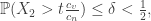
$\mathbb{P}(X_2>t\frac{c_v}{c_n})\leq \delta<\frac12,$

in fact for any $\delta<\frac12$ if we take $t$ large enough. But since

$\mathbb{P}(X_2>0)=\frac12(1-\mathbb{P}(X_2=0)),$

(which should in most cases be $\frac12$ ), this implies that $\frac{c_v}{c_n}$ cannot be very close to 0. In other words, $\frac{c_n}{c_v}$ is bounded above. This is in fact regularity enough to deduce that $c_n=n^{1/\alpha}$ from the Cauchy-type functional equation (*).

It remains to check that $\alpha\leq 2$ . Note that this equality case $\alpha=2$ corresponds exactly to the $\frac{1}{\sqrt{n}}$ scaling we saw for the normal distribution, in the context of the CLT. This motivates the proof. If $\alpha>2$ , we will show that the variance of X is finite, so CLT applies. This gives some control over $c_n$ in an $n\rightarrow\infty$ limit, which is plenty to ensure a contradiction.

To show the variance is finite, we use the definition of stable to check that there is a value of t such that

$\mathbb{P}(S_n>tc_n)<\frac14\,\forall n.$

Now consider the event that the maximum of the $X_i$ s is $>tc_n$ and that the sum of the rest is non-negative. This has, by independence, exactly half the probability of the event demanding just that the maximum be bounded below, and furthermore is contained within the event with probability $<\frac14$ shown above. So if we set

$z(n)=n\mathbb{P}(X>tc_n)$

we then have

$\frac14>\mathbb{P}(S_n>tc_n)\geq\frac12\mathbb{P}(\max X_i>tc_n)=\frac12[1-(1-\frac{z}{n})^n]$

$\iff 1-e^{-z(n)}\leq \frac12\text{ for large }n.$

So, $z(n)=n(1-F(tc_n))$ is bounded as $n$ varies. Rescaling suitably, this gives that

$x^\alpha(1-R(x))<M\,\forall x,\,\text{for some }M<\infty.$

This is exactly what we need to control the variance, as:

$\mathbb{E}X^2=\int_0^\infty \mathbb{P}(X^2>t)dt=\int_0^\infty \mathbb{P}(X^2>u^2)2udu$

$=\int_0^\infty 4u\mathbb{P}(X>u)du\leq \int_0^\infty 1\wedge\frac{4M}{u^{-(\alpha-1)}}du<\infty,$

using that X is symmetric and that $\alpha>2$ for the final equalities. But we know from CLT that if the variance is finite, we must have $\alpha=2$ .

All that remains is to mention how stable distributions fit into the context of limits in distribution of RVs. This is little more than a definition.

We say F is in the domain of attraction of a broadly stable distribution R if

$\exists a_n>0,b_n,\quad\text{s.t.}\quad \frac{S_n-b_n}{a_n}\stackrel{d}{\rightarrow}R.$

The role of $b_n$ is not hugely important, as a broadly stable distribution is in the domain of attraction of the corresponding strictly stable distribution.

The natural question to ask is: do the domains of attraction of stable distributions (for $0<\alpha\leq 2$ ) partition the space of probability distributions, or is some extra condition required?

Next time I will talk about stable distributions in a more analytic context, and in particular how a discussion of their properties is motivated by the construction of Levy processes.

Large Deviations and the CLT (eventuallyalmosteverywhere.wordpress.com)

Eventually Almost Everywhere

A blog about probability and olympiads by Dominic Yeo

Category Archives: Levy Processes