Means and Markov’s Inequality

The first time we learn what a mean is, it is probably called an average. The first time we meet it in a maths lesson, it is probably defined as follows: given a list of values, or possibilities, the mean is the sum of all the values divided by the number of such values.

This can be seen as both a probabilistic and a statistical statement. Ideally, these things should not be different, but at a primary school level (and some way beyond), there is a distinction to be drawn between the mean of a set of data values, say the heights of children in the class, and the mean outcome of rolling a dice. The latter is the mean of something random, while the former is the mean of something fixed and determined.

The reason that the same method works for both of these situations is that the distribution for the outcome of rolling a dice is uniform on the set of possible values. Though this is unlikely to be helpful to many, you could think of this as a consequence of the law of large numbers. The latter, performed jointly in all possible values says that you expect to have roughly equal numbers of each value when you take a large number of samples. If we refer to the strong law, this says that in fact we see this effect in the limit as we take increasingly large samples with probability one. Note that it is not trivial to apply LLN jointly to all values for a general continuous random variable. The convergence of sample distribution functions to the cdf of the underlying distribution is the content of the Glivenko-Cantelli Theorem.

In any case, this won’t work when there isn’t this symmetry where all values are equally likely. So in general, we have to define the mean of a discrete random variable as

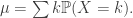
In other words, we are taking a sum of values multiplied by probabilities. By taking a suitable limit, a sum weighted by discrete probabilities converges to an integral weighted by a pdf. So this is a definition that will easily generalise.

Anyway, typically the next stage is to discuss the median. In the setting where we can define the mean directly as a sum of values, we must be given some list of values, which we can therefore write in ascending order. It’s then easy to define the median as the middle value in this ordered list. If the number of elements is odd, this is certainly well-defined. If the number is even, it is less clear. A lot of time at school was spent addressing this question, and the generally-agreed answer seemed to be that the mean of the middle two elements would do nicely. We shouldn’t waste any further time addressing this, as we are aiming for the continuous setting, where in general there won’t be discrete gaps between values in the support.

This led onwards to the dreaded box-and-whisker diagrams, which represent the min, lower quartile, median, upper quartile, and max in order. The diagram is structured to draw attention to the central points in the distribution, as these are in many applications of greater interest. The question of how to define the quartiles if the number of data points is not 3 modulo 4 is of exponentially less interest than the question of how to define the median for an even number of values, in my opinion. What is much more interesting is to note that the middle box of such a diagram would be finite for many continuous distributions with infinite support, such as the exponential distribution and the normal distribution.

Note that it is possible to construct any distribution as a function of a U[0,1] distribution by inverting the cdf. The box-and-whisker diagram essentially gives five points in this identification scheme.

Obviously, the ordered list definition fails to work for such distributions. So we need a better definition of median, which generalises. We observe that half the values are greater than the median, and so in a probabilistic setting, we say that the probability of being less than the median is equal to the probability of being greater. So we want to define it implicitly as:

So for a continuous distribution without atoms,

and this uniquely defines M.

The natural question to start asking is how this compares to the mean. In particular, we want to discuss the relative sizes. Any result about the possible relative values of the mean and median can be reversed by considering the negation of the random variable, so we focus on continuous random variables with non-negative support. If nothing else, these are the conditions for lots of data we might be interested in sampling in the ‘real world’.

It’s worth having a couple of questions to clarify what we are interested in. How about: is it possible for the mean to be 1000 times larger than the median; and is it possible for the median to be 1000 times larger than the mean?

The latter is easier to address. If the median is 1000 and the mean is 1, then with probability ½ the random variable X is at least 1000. So these values make a contribution to the mean of at least 500, while the other values make a contribution of at least zero (since we’ve demanded the RV be positive). This is a contradiction.

The former question turns out to be possible. The motivation should come from our box-and-whisker diagram! Once we have fixed the middle box, the median and quartiles are fixed, but we are free to fiddle with the outer regions as much as we like, so by making the max larger and larger, we can increase the mean freely without affecting the median. Perhaps it is clearest to view a discrete example: 1, 2, N. The median will always be 2, so we can increase N as much as desired to get a large mean.

The first answer is in a way more interesting, because it generalises to give a result about the tail of distributions. Viewing the median as the ½-quantile, we are saying that it cannot be too large relative to the mean. Markov’s inequality provides an identical statement about the general quantile. Instead of thinking about the constant a in an a-quantile, we look at values in the support.

Suppose we want a bound on for some positive a. Then if we define the function f by

so for all values. Hence the mean of f(X) is at most the mean of X. But the mean of f(X) can be calculated as

and so we conclude that

which is Markov’s Inequality.

It is worth remarking that this is trivially true when , since probabilities are always at most 1 anyway. Even beyond this region, it is generally quite weak. Note that it becomes progressively stronger if the contribution to the mean from terms greater than a is mainly driven by the contribution from terms close to a. So the statement is strong if the random variable has a light tail.

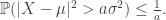
This motivates considering deviations from the mean, rather than the random variable itself. And to lighten the tail, we can square, for example, to consider the square distance from the mean. This version is Chebyshev’s Inequality:

Applying Markov an exponential function of a random variable is called a Chernoff Bound, and gives in some sense the bound on tails of a distribution obtained in this way.

Related articles

• “Memorylessness” property of some distributions. (zhengtianyu.wordpress.com)
• Stein’s Method (normaldeviate.wordpress.com)
• Probability: Exponential Random Variable (intellectualoutlet.wordpress.com)
• Catastrophes, Conspiracies, and Subexponential Distributions (Part II) (rigorandrelevance.wordpress.com)

Advertisement