Preferential Attachment Models

I’ve just read a really interesting paper by Peter Morters and Maren Eckhoff that made me feel I should look up some of the background and write a quick post. I may get onto some of the results in the paper at the end of this post, but I want to start by saying a bit about the model itself. I’ve spoken about this briefly in a previous post about several descriptions of complex networks, but I think it’s worth having a second attempt.

We seek a model for random graphs that gives a distribution which exhibits some of the properties of the sort of complex networks seen in the real world. In particular, whereas the degree distribution is Poisson, and so concentrated with exponential tails for the Erdos-Renyi random graph, data indicates that a better model for most applications would have power law tails for this degree distribution.

Albert and Barabasi propose growing such a graph via a so-called preferential attachment scheme. We start with some small possibly empty graph, and add new vertices one at a time. For each new vertex, we add exactly M edges between the new vertex and the vertices already present. The choice of these M other vertices is given by weighting by the degree of the (pre-existing) vertices. That is, vertices with large degree are more likely to be joined to new vertices. This is obviously designed to replicate some of the behaviour seen in say the formation of the internet, where new sites are more likely to link to established and popular sites (Google, Youtube and so on) than a uniformly chosen site.

This model has a couple of problems. Firstly, it is not immediately obvious how to start it. Obviously we need M vertices present for the PA dynamics to start working. In fact, whether one starts with a empty graph or a complete graph on M vertices makes little difference to the large n behaviour. Trickier is the question of multiple edges, which may emerge if we define the PA dynamics in the natural way, that is for each of the M edges in turn. Overcoming this is likely to be annoying.

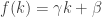
Bollobas and Riordan do indeed overcome this possible problems in a formal way, and prove that a version of this model does indeed have power law decay of the degree distribution, with exponent equal to 3. The model in the paper instead joins new vertex (n+1) to old vertex m with probability:

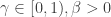
where f is some function, which for now we assume has the form . Since the vertices are constructed one at a time, it is well-defined to orient these edges from new to old vertices, hence this notion of in-degree makes sense.

It was not obvious to me that this model was more general than the Bollobas/Riordan model, but we will explain this in a little while. First I want to explain why the Bollobas/Riordan model has power law tails, and how one goes about finding the exponent of this decay, since this was presented as obvious in most of the texts I read yet is definitely an important little calculation.

So let’s begin with the Bollobas/Riordan model. It makes sense to think of the process in terms of time t, so there are t – M vertices in the graph. But if t is large, this is essentially equal to t. We want to track the evolution of the degree of some fixed vertex v_i, the ith vertex to be formed. Say this degree is d(t) at time t. Then the total number of edges in the graph at time t is roughly tM. Therefore, the probability that a new vertex gets joined to vertex v is roughly , where the M appears in the numerator because there are M fresh edges available. Note that we have ignored the possibility of trying to connect multiple edges from the new vertex to v, so this holds provided d is substantially smaller than t. With the boundary condition , this leads to the simple ODE

To me at least it was not immediately clear why this implied that the tail of the degree distribution had exponent 3. The calculation works as follows. Let D be the degree of a vertex at large time t, chosen uniformly at random.

Now we consider the Eckhoff / Morters model. The main difference here is that instead of assuming that each new vertex comes with a fixed number of edges, instead the new vertex joins to each existing vertex independently with probability proportional to the degree of the existing vertex. More precisely, they assume that edges are directed from new vertices to old vertices, and then each new vertex n+1 is joined to vertex m<n+1 with probability 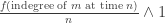, where , for .

I was stuck for a long time before I read carefully enough the assertion that . Of course, if this doesn’t hold, then the graph won’t grow fast enough. For, since the function f is now linear, we can lift the statement about evolution of the degree of a vertex to a statement about the evolution of the total number of edges. Note that each edge contributes exactly one to the total number of in-degrees. So we obtain

In particular, this is much less than t, so the majority of vertices have small degree. The answer is fairly clear in fact: since the preferential attachment mechanism depends only on in-degree, then if f(0)=0, since the in-degree of a new vertex will always be zero by construction, there is no way to get an additional edge to that vertex. So all the edges in the graph for large t will be incident to a vertex that had positive in-degree in the time 0 configuration. Hence we need for the model to be meaningful. Note that this means we effectively have a Erdos-Renyi type mechanism AND a preferential attachment evolution. As, for each new vertex, we add roughly edges to existing vertices chosen uniformly at random (rather than by a PA method) and also some assigned via PA. A previous paper by Dereich and Morters shows that the asymptotic degree distribution has a power law tail with exponent

Note that gives the same exponent (3) as the Bollobas / Riordan model.

We can apply a similar ODE approximation as above to estimate the likely large time behaviour of the number of edges:

So since , we have so defining F to be E(t)/t, we get:

       (1)

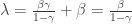
Noting that F’ is positive when and negative when suggests that for large t, this is an equilibrium point for F and hence . Obviously, this is highly non-rigorous, as F’ can be very small and still satisfy the relation (1), so it is not clear that the ‘equilibrium’ for F is stable. Furthermore, one needs to check that the binomial variables that supply the randomness to this model are sufficiently concentrated that this approximation by expectation is reasonable.

Nonetheless, as a heuristic this is not completely unsatisfactory, and it leads to the conclusion that E(t) is a linear function of t, and so the distribution of the out-degrees for vertices formed at large times t is asymptotically Poisson, with parameter

.

Note that this is the same situation as in Erdos-Renyi. In particular, it shows that all the power tail behaviour comes from the in-degrees. In a way this is unsurprising, as these evolve in time, whereas the out-degree of vertex t does not change after time t. Dereich and Morters formalise this heuristic with martingale analysis.

The reason we are interested in this type of model is that it better reflects models seen in real life. Some of these networks are organic, and so there it is natural to consider some form of random destructive mechanism, for example lightning, that kills a vertex and all its edges. We have to compare this sort of mechanism, which chooses a vertex uniformly at random, against a targeted attack, which deletes the vertices with largest degree. Note that in Erdos-Renyi, the largest degree is not much larger than the size of the typical degree, because the degree distribution is asymptotically Poisson. We might imagine that this is not the case in some natural networks. For example, if one wanted to destroy the UK power network, it would make more sense to target a small number of sub-stations serving large cities, than, say, some individual houses. However, a random attack on a single vertex is unlikely to make much difference, since the most likely outcome by far is that we lose only a single house etc.

In Eckhoff / Morters’ model, the oldest vertices are by construction have roughly the largest degree, so it is clear what targeting the most significant vertices means. They then show that these vertices include all the vertices that give the power law behaviour. In particular, if you remove all of these vertices and, obviously, the edges incident to them, you are left with a graph with exponential tail in the asymptotic degree distribution, with largest degree on the order of log n. It was shown in a previous paper that this type of network is not vulnerable to random removal of nodes. Perhaps most interestingly, these authors now prove that after removing the most significant vertices, the network IS now vulnerable to random removal of nodes, leading to the conclusion that it is preferable to experience a random attack followed by a targeted attack than vice versa!

In a future (possibly distant) post, I want to say some slightly more concrete things about how these processes link to combinatorial stochastic processes I understand slightly better, in particular urn models. I might also discuss the configuration model, an alternative approach to generating complex random networks.

Related articles

• How much is the stacks project graph like a random graph? (quomodocumque.wordpress.com)
• Three properties of real-world graphs (johndcook.com)
• Graph Project (marscoding.wordpress.com)
• How many people do you know? (rockndata.wordpress.com)
• Graph matching & Levenshtein distance (p1) (alikhuram.wordpress.com)

Advertisement