This post is motivated by G(N,p), the classical Erdos-Renyi random graph, specifically its critical window, when  .
.
We start with the following observation, which makes no restriction on p. Suppose a component of G(N,p) is a tree. Then, the graph geometry of this component is that of a uniform random tree on the appropriate number of vertices. This is deliberately informal. To be formal, we’d have to say “condition on a particular subset of vertices forming a tree-component” and so on. But the formality is broadly irrelevant, because at the level of metric scaling limits, if we want to describe the structure of a tree component, it doesn’t matter whether it has  or
or  vertices, because in both cases the tree structure is uniform. The only thing that changes is the scaling factor.
In general, when V vertices form a connected component of a graph with E edges, we define the excess to be E-V+1. So the excess is non-negative, and is zero precisely when the component is a tree. I’m reluctant to say that the excess counts the number of cycles in the component, but certainly it quantifies the amount of cyclic structure present. We will sometimes, in a mild abuse of notation, talk about excess edges. But note that for a connected component with positive excess, there is a priori no way to select which edges would be the excess edges. In a graph process, or when there is some underlying exploration of the component, there sometimes might be a canonical way to classify the excess edges, though it’s worth remarking that the risk of size-biasing errors is always extremely high in this sort of situation.
Returning to the random graph process, as so often there are big changes around criticality. In the subcritical regime, the components are small, and most of them, even the largest with high probability, are trees. In the supercritical regime, the giant component has excess  , which is qualitatively very different.
It feels like every talk I’ve ever given has begun with an exposition of Aldous’s seminal paper [Al97] giving a distributional scaling limit of the sizes of critical components in the critical window, and a relation between the process on this time-scale and the multiplicative coalescent. And it remains relevant here, because the breadth-first exploration process can also be used to track the number of excess edges.
In a breadth-first exploration, we have a stack of vertices we are waiting to explore. We pick one and look its neighbours restricted to the rest of the graph, that is without the vertices we have already fully explored, and also without the other vertices in the stack. That’s the easiest way to handle the total component size. But we can simultaneously track how many times we would have joined to a neighbour within the stack, which leads to an excess edge, and Aldous derives a joint distributional scaling limit for the sizes of the critical components and their excesses. (Note that in this case, there is a canonical notion of excess edge, but it depends not just on the graph structure, but also on the extra randomness of the ordering within the breadth-first search.)
Roughly speaking, we consider the reflected exploration process, and its scaling limit, which is a reflected parabolically-drifting Brownian motion (though the details of this are not important at this level of exposition, except that it’s a well-behaved non-negative process that hits zero often). The component sizes are given by the widths of the excursions above zero, scaled up in a factor  . Then conditional on the shape of the excursion, the excess is Poisson with parameter the area under the excursion, with no rescaling. That is, a critical component has
  excess.
So, with Aldous’s result in the background, when we ask about the metric structure of these critical components, we are really asking: “what does a uniformly-chosen connected component with fixed excess look like when the number of vertices grows?”
I’ll try to keep notation light, but let’s say T(n,k) is a uniform choice from connected graphs on n vertices with excess k.
[Note, the separation of N and n is deliberate, because in the critical window, the connected components have size  , so I want to distinguish the two problems.]
In this post, we will mainly address the question: “what does the cycle structure of T(n,k) look like for large n?” When k=0, we have a uniform tree, and the convergence of this to the Brownian CRT is now well-known [CRT2, LeGall]. We hope for results with a similar flavour for positive excess k.
2-cores and kernels
First, we have to give a precise statement of what it means to study just the cycle structure of a connected component. From now on I will assume we are always working with a connected graph.
There are several equivalent definitions of the 2-core C(G) of a graph G:
- When the excess is positive, there are some cycles. The 2-core is the union of all edges which form part of some cycle, and any edges which lie on a path between two edges which both form part of some cycle.
- C(G) is the maximal induced subgraph where all degrees are at least two.
- If you remove all the leaves from the graph, then all the leaves from the remaining graph, and continue, the 2-core is the state you arrive at where there are no leaves.
It’s very helpful to think of the overall structure of the graph as consisting of the 2-core, with pendant trees ‘hanging off’ the 2-core. That is, we can view every vertex of the 2-core as the root of a (possibly size 1) tree. This is particular clear if we remove all the edges of the 2-core from the graph. What remains is a forest, with one tree for each vertex of the 2-core.

In general, the k-core is the maximal induced subgraph where all degrees are at least k. The core is generally taken to be something rather different. For this post (and any immediate sequels) I will never refer to the k-core for k>2, and certainly not to the traditional core. So I write ‘core’ for ‘2-core’.
As you can see in the diagram, the core consists of lots of paths, and topologically, the lengths of these paths are redundant. So we will often consider instead the kernel, K(G), which is constructed by taking the core and contracting all the paths between vertices of degree greater than 2. The resulting graph has minimal degree at least three. So far we’ve made no comment about the simplicity of the original graphs, but certainly the kernel need not be simple. It will regularly have loops and multiple edges. The kernel of the graph and core in the previous diagram is therefore this:

Kernels of critical components
To recap, we can deconstruct a connected graph as follows. It has a kernel, and each edge of the kernel is a path length of some length in the core. The rest of the graph consists of trees hanging off from the core vertices.
For now, we ask about the distribution of the kernel of a T(n,K). You might notice that the case k=1 is slightly awkward, as when the core consists of a single cycle, it’s somewhat ambiguous how to define the kernel. Everything we do is easily fixable for k=1, but rather than carry separate cases, we handle the case  .
.
We first observe that fixing k doesn’t confirm the number of vertices or edges in the kernel. For example, both of the following pictures could correspond to k=3:

However, with high probability the kernel is 3-regular, which suddenly makes the previous post relevant. As I said earlier, it can introduce size-biasing errors to add the excess edges one-at-a-time, but these should be constant factor errors, not scaling errors. So imagine the core of a large graph with excess k=2. For the sake of argument, assume the kernel has the dumbbell / handcuffs shape. Now add an extra edge somewhere. It’s asymptotically very unlikely that this is incident to one of the two vertices with degree three in the core. Note it would need to be incident to both to generate the right-hand picture above. Instead, the core will gain two new vertices of degree three.
Roughly equivalently, once the size of the core is fixed (and large) we have to make a uniform choice from connected graphs of this size where almost every vertex has degree 2, and of the rest have degree 3 or higher. But the sum of the degrees is fixed, because the excess is fixed. If there are n vertices in the core, then there are  more graphs where all the vertices have degree 2 or 3, than graphs where a vertex has degree at least 4. Let’s state this formally.
Proposition: The kernel of a uniform graph with n vertices and excess is, with high probability as  , 3-regular.
This proved rather more formally as part of Theorem 7 of [JKLP], essentially as a corollary after some very comprehensive generating function setup; and in [LPW] with a more direct computation.
In the previous post, we introduced the configuration model as a method for constructing regular graphs (or any graphs with fixed degree sequence). We observe that, conditional on the event that the resulting graph is simple, it is in fact uniformly-distributed among simple graphs. When the graph is allowed to be a multigraph, this is no longer true. However, in many circumstances, as remarked in (1.1) of [JKLP], for most applications the configuration model measure on multigraphs is the most natural.
Given a 3-regular labelled multigraph H with 2(k-1) vertices and 3(k-1) edges, and K a uniform choice from the configuration model with these parameters, we have

where t(H) is the number of loops in H, and mult(e) the multiplicity of an edge e. This might seem initially counter-intuitive, because it looks we are biasing against graphs with multiple edges, when perhaps our intuition is that because there are more ways to form a set of multiple edges we should bias in favour of it.

I think it’s most helpful to look at a diagram of a multigraph as shown, and ask how to assign stubs to edges. At a vertex with degree three, all stub assignments are different, that is 3!=6 possibilities. At the multiple edge, however, we care which stubs match with which stubs, but we don’t care about the order within the multi-edge. Alternatively, there are three choices of how to divide each vertex’s stubs into (2 for the multi-edge, 1 for the rest), and then two choices for how to match up the multi-edge stubs, ie 18 in total = 36/2, and a discount factor of 2.
We mention this because in fact K(T(n,k)) converges in distribution to this uniform configuration model. Once you know that K(T(n,k)) is with high probability 3-regular, then again it’s probably easiest to think about the core, indeed you might as well condition on its total size and number of degree 3 vertices. It’s then not hard to convince yourself that a uniform choice induces a uniform choice of kernel. Again, let’s state that as a proposition.
Proposition: For any H a 3-regular labelled multigraph H with 2(k-1) vertices and 3(k-1) edges as before,

As we said before, the kernel describes the topology of the core. To reconstruct the graph, we need to know the lengths in the core, and then how to glue pendant trees onto the core. But this final stage depends on k only through the total length of paths in the core. Given that information, it’s a combinatorial problem, and while I’m not claiming it’s easy, it’s essentially the same as for the case with k=1, and is worth treating separately.
It is worth clarifying a couple of things first though. Even the outline of methods above relies on the fact that the size of the core diverges as n grows. Again, the heuristic is that up to size-biasing errors, T(n,k) looks like a uniform tree with some uniformly-chosen extra edges. But distances in T(n,k) scale like  (and thus in critical components of G(N,p) scale like ). And the core will be roughly the set of edges on paths between the uniformly-chosen pairs of vertices, and so will also have length
  .
.
Once you have conditioned on the kernel structure, and the (large) number of internal vertices on paths in the core (ie the length of the core), it is natural that the assignment of the degree-2 vertices to core paths / kernel edges is uniform. A consequence of this is that if you record  the lengths of paths in the core, where m=3(k-1), then
This is stated formally as Corollary 7 b) of [ABG09]. It’s worth noting that this confirms that the lengths of core paths are bounded in probability away from zero after the appropriate rescaling. In seeking a metric scaling limit, this is convenient as it means there’s so danger that two of the degree-3 vertices end up in ‘the same place’ in the scaling limit object.
To recap, the only missing ingredients now to give a complete limiting metric description of T(n,k) are 1) a distributional limit of the total core length; 2) some appropriate description of set of pendant trees conditional on the size of the pendant forest. [ABG09] show the first of these. As remarked before, all the content of the second of these is encoded in the unicyclic k=1 case, which I have written about before, albeit slightly sketchily, here. (Note that in that post we get around size-biasing by counting a slightly different object, namely unicyclic graphs with an identified cyclic edge.)
However, [ABG09] also propose an alternative construction, which you can think of as glueing CRTs directly onto the stubs of the kernel (with the same distribution as before). The proof that this construction works isn’t as painful as one might fear, and allows a lot of the other metric distributional results to be read off as corollaries.
References
[ABG09] – Addario-Berry, Broutin, Goldschmidt – Critical random graphs: limiting constructions and distributional properties
[CRT2] – Aldous – The continuum random tree: II
[Al97] – Aldous – Brownian excursions, critical random graphs and the multiplicative coalescent
[JKLP] – Janson, Knuth, Luczak, Pittel – The birth of the giant component
[LeGall] – Le Gall – Random trees and applications
[LPW] – Luczak, Pittel, Wierman – The structure of a random graph at the point of the phase transition


![\mathbb{E}[X|A]\ge \mathbb{E}[X]](https://s0.wp.com/latex.php?latex=%5Cmathbb%7BE%7D%5BX%7CA%5D%5Cge+%5Cmathbb%7BE%7D%5BX%5D&bg=ffffff&fg=333333&s=0&c=20201002)

, for which we showed that all the components are small, in the sense that
, although the same argument would also give
with high probability if we used stronger Chernoff bounds;
, for which there is a unique giant component , ie that
, the survival probability of a Galton-Watson branching process with Poisson(
) offspring distribution. Arguing for example by a duality argument shows that with high probability all other components are small in the same sense as in the subcritical regime.


 and let
  be a sequence of non-negative integers such that
  is even. Then the configuration model with degree sequence d is a random multigraph with vertex set [n], constructed as follows:
![i\in[n]](https://s0.wp.com/latex.php?latex=i%5Cin%5Bn%5D&bg=ffffff&fg=333333&s=0&c=20201002) , assign
, assign  half-edges;
 , in which, by construction, vertex i has degree

 is the multiplicity with which a given edge e appears in H.
 , the d-regular configuration model
  .
. will consist of n/2 disjoint edges.
 will consist of some number of disjoint cycles, and it is a straightforward calculation to check that when n is large, with high probability the graph will be disconnected.
 is connected with high probability. This is, in fact, a very weak result, since in fact
  [Bol81, Wor81]. Here, d-connected means that one must remove at least d vertices in order to disconnect the graph, or, equivalently, that there are d disjoint paths between any pair of vertices. Furthermore, Bollobas shows that for
  satisfies

 vertices, with
  , and with no edges between the classes is
 . We will refer to a
  symmetric matrix with non-negative entries as a kernel.
 and a vector
  satisfying
  , and
, and  a kernel, we define the inhomogeneous random graph
  with k types as:
 vertices have type i.
 (for
(for ![v\ne w\in [n]](https://s0.wp.com/latex.php?latex=v%5Cne+w%5Cin+%5Bn%5D&bg=ffffff&fg=333333&s=0&c=20201002) ) is present, independently, with probability
) is present, independently, with probability
 have type 1,
  have type 2, etc etc. This makes no difference except in terms of the notation we have to use if we want to use exchangeability arguments later.
 on [k], and assigns the types of the vertices of [n] in an IID fashion according to
  . The exponential form has a more natural interpretation if we ever need to turn the IRGs into a process. Additionally, it avoids the requirement to treat small values of n (for which, a priori,
  might be greater than 1) separately.
 .
. for which
  , where
 ![\pi=(\pi_1,\ldots,\pi_k)\in[0,1]^k](https://s0.wp.com/latex.php?latex=%5Cpi%3D%28%5Cpi_1%2C%5Cldots%2C%5Cpi_k%29%5Cin%5B0%2C1%5D%5Ek&bg=ffffff&fg=333333&s=0&c=20201002) satisfies
satisfies  .
. be a uniformly-chosen vertex in [n]. Clearly
  , with the immediate mild notation abuse of viewing
  :
: , the number of type j neighbours of
  .
. .
.![p_j\left[1-\exp\left(-\frac{\kappa_{i,j}}{n}\right)\right]\approx \frac{p_j\cdot \kappa_{i,j}}{n} \approx \kappa_{i,j}\pi_j](https://s0.wp.com/latex.php?latex=p_j%5Cleft%5B1-%5Cexp%5Cleft%28-%5Cfrac%7B%5Ckappa_%7Bi%2Cj%7D%7D%7Bn%7D%5Cright%29%5Cright%5D%5Capprox+%5Cfrac%7Bp_j%5Ccdot+%5Ckappa_%7Bi%2Cj%7D%7D%7Bn%7D+%5Capprox+%5Ckappa_%7Bi%2Cj%7D%5Cpi_j&bg=ffffff&fg=333333&s=0&c=20201002) , and similarly in the case j=i, so in both cases, the number of neighbours of type j is distributed approximately as
, and similarly in the case j=i, so in both cases, the number of neighbours of type j is distributed approximately as  .
. .
.
 offspring distribution, as we’ve used informally earlier in the course.
 . At a heuristic level, we imagine that all vertices whose local neighbourhood is ‘infinite’ are in fact part of the same giant component, which should occupy
  vertices. In its most basic form, the result is
 (*)
(*) , then each time we add a new edge (such an argument is often called ‘sprinkling‘), the probability that these two components are joined is
  , and so if we add lots of edges (which happens as we move from edge probability
  ) then with high probability these two components get joined.
 and
and  ) and then show that all larger components are the same by a joint exploration process or a technical sprinkling argument. Cf the books of Bollobas and of Janson, Luczak, Rucinski. See also
  ,
, with high probability as
  with high probability.
 , and the same approximation remains valid as we explore the graph (for example in a breadth-first fashion) either until we have seen a large number of vertices, or unless some ultra-pathological event happens, such as a vertex having degree n/3.
 offspring, and in this lecture and the next we try to make this notion precise, and discuss some consequences when we can show that this form of convergence occurs.
 , where the vertex set of
  is [n], or certainly increasing in n (as in the first example).
 , we say such a sequence
  , we have
  . In words, the neighbourhood around
  in
in  in
in  , so long as n is large enough (for given r).
 , the binary tree to depth n.
 . Slightly less obviously, if we take
  with nearest-neighbour edges, and where each vertex
  , as shown below:
 ,
,
 , the path of length n. Then, the r-neighbourhood of a vertex is isomorphic to
  , unless that vertex is within graph-distance (r-1) of one of the leaves of
  , from which we conclude the unsurprising result that
  converges in the local weak sense to
  . (Which is vertex-transitive, so it doesn’t matter where we select the root.)
 be the set of leaves of
  converges in distribution. Indeed,
 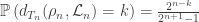 , whenever
  , and so the given distance converges in distribution to the Geometric distribution with parameter 1/2 supported on {0,1,2,…}.
 . This is easiest if we have constructed the Galton-Watson tree as a subset of the infinite Ulam-Harris tree, where vertices have labels like (3,5,17,4), whose parent is (3,5,17). If this child vertex is part of the tree, then so are (3,5,17,1), (3,5,17,2), and (3,5,17,3). This means our breadth-first order is canonically well-defined, as we have a natural ordering of the children of each parent vertex.
![\mu=\mathbb{E}[X]>1](https://s0.wp.com/latex.php?latex=%5Cmu%3D%5Cmathbb%7BE%7D%5BX%5D%3E1&bg=ffffff&fg=333333&s=0&c=20201002) .
. given by
 is the number of children of
  . In this way, we see that
 , and so the condition that
  requires
 .
. be a random walk with
  and IID increments
  satisfying
  . Let
. Let  be the hitting time of -k.
 .
. . The goal for today was to give a self-contained proof of the result that in the subcritical setting
![v\in[n]](https://s0.wp.com/latex.php?latex=v%5Cin%5Bn%5D&bg=ffffff&fg=333333&s=0&c=20201002) outwards from v, at all times the number of ‘children’ of v which haven’t already been considered is ‘at most’
outwards from v, at all times the number of ‘children’ of v which haven’t already been considered is ‘at most’  . Since, for example, if we already know that eleven vertices, including the current one w are in C(v), then the distribution of the number of new vertices to be added to consideration because they are directly connected to w has conditional distribution
  .
. , and also that, so long as we don’t replace 11 by a linear function of n, that
 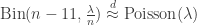 .
. on the same probability space with correct marginals, that is
 , we always have the option to couple with a uniform U(0,1) random variable. That is, when
 ![U\sim U[0,1]](https://s0.wp.com/latex.php?latex=U%5Csim+U%5B0%2C1%5D&bg=ffffff&fg=333333&s=0&c=20201002) , we have
, we have  , where the inverse of the distribution function is defined (in the non-obvious case of atoms) as
 . This coupling can be used simultaneously on two random variables X and Y, as
  , to generate a coupling of X and Y.
 ,
, . This is particularly clear in the case of discrete measures, as then
 and
and  are distance 1 apart (the maximum) for all values of n. Similarly, the uniform distribution on [0,1] and the uniform distribution on
  are also distance 1 apart.
 satisfies
  , and there exists a coupling such that equality is achieved.
  . In the end, we showed that when
  is any diverging sequence, and
 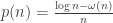 , then we have that G(n,p(n)) is with high probability not connected.
 , and show that for this range of p, the graph G(n,p(n)) is with high probability connected.
 , or whatever scaling turns out to be convenient for the proof, but conclude the result for all diverging
  , we use a second-moment method argument to establish that G(n,p) contains an isolated vertex with high probability. Note that a given vertex v is isolated precisely if n-1 edges are not present. Furthermore, two given vertices v,w are both isolated, precisely if 2n-3 edges are not present. So in fact, both the first moment and the second moment of the number of isolated vertices are straightforward to evaluate.
 , satisfies
![\mathbb{E}[Y_n]= \exp(\omega(n)+o(1))\rightarrow\infty.](https://s0.wp.com/latex.php?latex=%5Cmathbb%7BE%7D%5BY_n%5D%3D+%5Cexp%28%5Comega%28n%29%2Bo%281%29%29%5Crightarrow%5Cinfty.&bg=ffffff&fg=333333&s=0&c=20201002) (*)
(*)![\mathrm{Var}(Y_n)= (1+o(1))\mathbb{E}[Y_n],](https://s0.wp.com/latex.php?latex=%5Cmathrm%7BVar%7D%28Y_n%29%3D+%281%2Bo%281%29%29%5Cmathbb%7BE%7D%5BY_n%5D%2C&bg=ffffff&fg=333333&s=0&c=20201002)
 .
. requires only a first-moment method, it is more technical because it involves the non-clear direction of the informal equivalence:
 citations towards one of Erdos and Renyi’s original papers on the topic.
 we claim:
 as
as 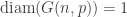 , then
  , the complete graph on n vertices. In other words, every possible edge is actually present. But the probability of this event is
  , so long as p<1.
 . We use a union bound, where we study the probability that the graph distance
  for two fixed vertices
  first, and then sum over all such pairs. Of course, there is a probability p that the two vertices are directly connected by an edge. Then, there are (n-2) other vertices with the potential to be a common neighbour of v and w, which would ensure that the graph distance between them is at most two. So
![\mathbb{P}(d_{G(n,p)}(v,w)>2)=(1-p)[1-p^2]^{n-2} .](https://s0.wp.com/latex.php?latex=%5Cmathbb%7BP%7D%28d_%7BG%28n%2Cp%29%7D%28v%2Cw%29%3E2%29%3D%281-p%29%5B1-p%5E2%5D%5E%7Bn-2%7D+.&bg=ffffff&fg=333333&s=0&c=20201002)
![\mathbb{P}(\mathrm{diam}(G(n,p)) >2) \le \sum_{v\ne w \in[n]} \mathbb{P}(d_{G(n,P)}(v,w)>2)](https://s0.wp.com/latex.php?latex=%5Cmathbb%7BP%7D%28%5Cmathrm%7Bdiam%7D%28G%28n%2Cp%29%29+%3E2%29+%5Cle+%5Csum_%7Bv%5Cne+w+%5Cin%5Bn%5D%7D+%5Cmathbb%7BP%7D%28d_%7BG%28n%2CP%29%7D%28v%2Cw%29%3E2%29&bg=ffffff&fg=333333&s=0&c=20201002)
![\le \binom{n}{2} (1-p)[1-p^2]^{n-2} \rightarrow 0,](https://s0.wp.com/latex.php?latex=%5Cle+%5Cbinom%7Bn%7D%7B2%7D+%281-p%29%5B1-p%5E2%5D%5E%7Bn-2%7D+%5Crightarrow+0%2C&bg=ffffff&fg=333333&s=0&c=20201002)
 we have
 as
as 


 , we have
  , and overall we obtain
![\mathbb{P}(E(G(n,p))\text{ not a matching}) \le \sum_{v\in[n]} \mathbb{P}(\mathrm{deg}_{G(n,p)}(v)\ge 2)](https://s0.wp.com/latex.php?latex=%5Cmathbb%7BP%7D%28E%28G%28n%2Cp%29%29%5Ctext%7B+not+a+matching%7D%29+%5Cle+%5Csum_%7Bv%5Cin%5Bn%5D%7D+%5Cmathbb%7BP%7D%28%5Cmathrm%7Bdeg%7D_%7BG%28n%2Cp%29%7D%28v%29%5Cge+2%29&bg=ffffff&fg=333333&s=0&c=20201002)


