I am aiming to write a short post about each lecture in my ongoing course on Random Graphs. Details and logistics for the course can be found here.
Preliminary – positive correlation, Harris inequality
I wrote about independence, association, and the FKG property a long time ago, while I was still an undergraduate taking a first course on Percolation in Cambridge. That post is here. In the lecture I discussed the special case of the FKG inequality applied in the setting of product measure setting, of which the Erdos-Renyi random graph is an example, and which is sometimes referred to as the Harris inequality.
Given two increasing events A and B, say for graphs on [n], then if  is product measure on the edge set, we have

Intuitively, since both A and B are ‘positively-correlated’ with the not-rigorous notion of ‘having more edges’, then are genuinely positively-correlated with each other. We will use this later in the post, in the form ![\mathbb{E}[X|A]\ge \mathbb{E}[X]](https://s0.wp.com/latex.php?latex=%5Cmathbb%7BE%7D%5BX%7CA%5D%5Cge+%5Cmathbb%7BE%7D%5BX%5D&bg=ffffff&fg=333333&s=0&c=20201002) , whenever X is an increasing RV and A is an increasing event.
, whenever X is an increasing RV and A is an increasing event.
The critical window
During the course, we’ve discussed separately the key qualitative features of the random graph  in the
- subcritical regime when
 , for which we showed that all the components are small, in the sense that
  , although the same argument would also give
 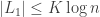 with high probability if we used stronger Chernoff bounds;
- supercritical regime when
 , for which there is a unique giant component , ie that
  , the survival probability of a Galton-Watson branching process with Poisson(
 ) offspring distribution. Arguing for example by a duality argument shows that with high probability all other components are small in the same sense as in the subcritical regime.
In between, of course we should study  , for which it was known that
 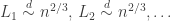 . (*) That is, the largest components are on the scale
  , and there are lots of such critical components.
In the early work on random graphs, the story ended roughly there. But in the 80s, these questions were revived, and considerable work by Bollobas and Luczak, among many others, started investigating the critical setting in more detail. In particular, between the subcritical and the supercritical regimes, the ratio  between the sizes of the largest and second-largest components goes from ‘concentrated on 1’ to ‘concentrated on 0’. So it is reasonable to ask what finer scaling of the edge probability
  around
  should be chosen to see this transition happen.
Critical window
In this lecture, we studied the critical window, describing sequences of probabilities of the form
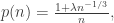
where  . (Obviously, this is a different use of to previous lectures.)
It turns out that as we move from  to
to  , this window gives exactly the right scaling to see the transition of described above. Work by Bollobas and Luczak and many co-authors and others in the 80s establish a large number of results in this window, but for the purposes of this course, this can be summarised as saying that the critical window has the same scaling behaviour as
  , with a large number of components on the scale
  (see (*) earlier), but different scaling limits.
Note: Earlier in the course, we have discussed local limits, in particular for  , where the local limit is a Galton-Watson branching process tree with offspring distribution
  . Such local properties are not sufficient to distinguish between different probabilities within the critical window. Although there are lots of critical components, it remains the case that asymptotically almost all vertices are in ‘small components’.
The precise form of the scaling limit for

as  was shown by Aldous in 1997, by lifting a scaling limit result for the exploration process, which was discussed in this previous lecture and this one too. Since Brownian motion lies outside the assumed background for this course, we can’t discuss that, so this lecture establishes upper bounds on the correct scale of
  in the critical window. Precisely, we will show the following proposition:
Proposition 1: fix  , and let
 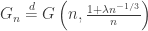 . Then

Proof: In the lecture, we gave a quick proof of the case  by a direct comparison of the exploration process with the exploration process of a branching process whose offspring distribution is binomial and has expectation
  .
.
It remains to handle the case  , though the argument which follows works for general . As before, we want to study the exploration process. In order to have a component of size at least
  , the exploration process must stay above its running minimum for at least steps. (**)
The drift of the exploration process may initially be positive (in fact it will be approximately  ), but the drift is decreasing in time, and is certainly negative when
  , so for large $K$ the event at (**) is indeed unlikely. In addition, when we formalise this we will find studying the entire exploration process hard, but are motivated by the idea that most large components should be explored early in the process.
[In what follows, one should really replace most instances of with  , and so on.]
Fix a small constant  , and define the events


Then the key observation is that

To see this, note that if  does not hold, then certainly
  components have been explored before vertex . Therefore, if we are exploring
  during vertex , then
  holds, and if we are yet to explore , then
  holds. If we demand
  , then it is not possible that this component has already been explored.
To handle  , we use a stochastic bounding argument similar to ones deployed before. In this setting, we note that conditional on any values of
  , we have

but when  , we have the stronger bound

We can therefore obtain upper bounds on ![\mathbb{E}\left[S_{Kn^{2/3}}\right]](https://s0.wp.com/latex.php?latex=%5Cmathbb%7BE%7D%5Cleft%5BS_%7BKn%5E%7B2%2F3%7D%7D%5Cright%5D&bg=ffffff&fg=333333&s=0&c=20201002) , and also second-moment control, enabling us to use Chebyshev’s inequality to deduce
, and also second-moment control, enabling us to use Chebyshev’s inequality to deduce

(The details of this calculation is one of the starred exercises.)
To proceed, we update the key observation as

The middle of these is now easy to handle. Each time the exploration process ‘starts’ a new component, it does so by choosing an unexplored vertex uniformly at random. Therefore, conditional on  (an event which depends on the random graph, not on the randomness deciding the order of the components), the number of components explored before is stochastically dominated by
  , ie
, ie 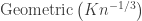 . [Here the geometric distribution is supported on {0,1,2,…} .]
In particular, the conditional expectation of this quantity is bounded above by  , and so

whenever  , and so in particular

Finally, we turn to  , for which we use FKG to handle the graph
  with its largest component
  removed. Conditional on
  , we have

conditioned such that  . That is, the remaining graph is an Erdos-Renyi random graph with the same probability, but conditioned such that its largest component is not too large.
In any case, so every possible value of , this is a decreasing event, and so we may apply FKG / Harris to deduce that
![\mathbb{E}\left[ |C(v)|\text{ in }G_n\backslash L_1(G_n)\,\big|\, |L_1(G_n)|\right] \le \mathbb{E}\left[ |C(v)|\text{ in }G(n-|L_1|,p)\,\big|\, |L_1(G_n)|\right],](https://s0.wp.com/latex.php?latex=%5Cmathbb%7BE%7D%5Cleft%5B+%7CC%28v%29%7C%5Ctext%7B+in+%7DG_n%5Cbackslash+L_1%28G_n%29%5C%2C%5Cbig%7C%5C%2C+%7CL_1%28G_n%29%7C%5Cright%5D+%5Cle+%5Cmathbb%7BE%7D%5Cleft%5B+%7CC%28v%29%7C%5Ctext%7B+in+%7DG%28n-%7CL_1%7C%2Cp%29%5C%2C%5Cbig%7C%5C%2C+%7CL_1%28G_n%29%7C%5Cright%5D%2C&bg=ffffff&fg=333333&s=0&c=20201002)
and this expectation can again be controlled by comparing with the expected total population size of a binomial branching process. In particular, when is large, this branching process is subcritical, and the expected total population size is finite (though  ).
).
We skip the details of this estimate in this blog post, but crucially we can iterate this argument across all components explored before the largest component, the number of which remains stochastically bounded by a geometric RV as before. We obtain
![\mathbb{E}\left[\text{vertices explored before }L_1\,\big|\, |L_1|> Kn^{2/3}\right] \le \frac{n^{2/3}}{K(K-\lambda)},](https://s0.wp.com/latex.php?latex=%5Cmathbb%7BE%7D%5Cleft%5B%5Ctext%7Bvertices+explored+before+%7DL_1%5C%2C%5Cbig%7C%5C%2C+%7CL_1%7C%3E+Kn%5E%7B2%2F3%7D%5Cright%5D+%5Cle+%5Cfrac%7Bn%5E%7B2%2F3%7D%7D%7BK%28K-%5Clambda%29%7D%2C&bg=ffffff&fg=333333&s=0&c=20201002)
whenever  , and so by Markov we again have

The proposition then follows by a union bound.

