Finitely many solutions

This post is aimed at secondary-school students pitched roughly at the level of the British Mathematical Olympiad. It is ostensibly about a certain class of number theory problems, but the main underlying mathematical principle is broader than this. The post is based on an in-person session I have given to students and at teachers’ conferences a few times over the past five years, but I’ve chosen to write it up at this moment because of the connection to Problem 4 on the most recent BMO1 paper, which we discuss later in the post.

Prologue

Alice and Bob make the following statements:

• Alice: all prime numbers are odd.
• Bob: we can’t say anything about whether prime numbers are odd or even.

These are different types of statement, one objective, one more subjective; but both are wrong. Alice is wrong because 2 is a prime, and 2 is of course even. Bob is wrong because while Alice is wrong, and the alternative statement “all prime numbers are even” is even more wrong¹, there are plenty of possible statements that are true and useful, including

• Cleo: all prime numbers are odd except 2.

and weaker versions (that may be more relevant in other contexts) like “all primes greater than are odd”.

The characters now turn their attention to another family of integers, the square numbers , and the sixth powers

• Alice: no square numbers are prime.
• Bob: I agree.
• Alice: most square numbers are not sixth powers.
• Bob: hang on, but infinitely many square numbers are sixth powers?

The difficulty in the second statement is what does most mean in this context? The square of an integer n is a sixth power if and only if n is a cube, and so Alice’s statement is equivalent to the statement “most positive integers are not cubes”, which is intuitively reasonable, but would require more clarification than the analogous statement “most primes are odd”. Is it not relevant, for example, that 1/4 of the first eight positive integers are in fact cubes?

It is not impossible to formalise this notion of most in a reasonable way to permit the two statements above².

But the bulk of this post will discuss situations that extend the first of these conversations, ie when it’s not true to say “all element of X have property Y”, but where it’s nonetheless possible to make a useful intermediate statement.

Warmup problems

I hope most readers know how to solve an equation such as

and indeed learning how to solve such equations forms a important milestone in mathematical education as the first example of various principles of algebra. When such equations are still novel, teachers would be advised to avoid examples such as

for which the answers are, respectively, ‘no solutions’ and ‘every x satisfies this’. While they are perfectly valid equations, it means something slightly different to solve them, since the answer set has different structure and, more importantly, the method is different since it doesn’t consist of a sequence of a manipulations leading directly to the required conclusion .

However, I mention this in passing to clarify that even in the simplest possible family of equations (probably encountered somewhere between ages 9 and 13) we are mindful that not all equations have unique solutions.

I’ve adapted a problem from the American competition AIME:

Find all integers such that is a prime.

One could start by writing if you wish, but in fact we only need to work with the left hand side, so it’s better to avoid this if possible. The key to this problem is to avoid the prime condition initially, and just manipulate the LHS until it simplifies as

(*)

which is never a prime, since is a square number and so, as already discussed, never a prime.

So at a meta-level, comparing with the other problem in this section, this one also begins with reversible algebraic manipulations, but does not end with a direct reduction to , and indeed the final step is not reversible at all.

Finally, we remark that the original version of the AIME problem was

Prove that for all integers , is a perfect square.

The same algebraic reduction as (*) resolves the original version without an extra step concerning primes.

To be, or not to be, a perfect square

The rest of this article will focus entirely on problems of the form: find all positive integers n such that […] is a perfect square.

As setup, we’ll always consider a function f(n), and the sequence f(1),f(2),f(3),… and the question, comment on the set of n is f(n) a square? In particular, this is a more open-ended question than for which n is f(n) a square, which requires a more exact answer. We’ll aim for one of the following possible answers:

• f(n) is always a square;
• f(n) is a square for infinitely many n;
• f(n) is a square for only finitely many n;
• f(n) is never a square.

Clearly this is not an exhaustive list of possible descriptions³ of the set under discussion, but it will do for now. The difference between the second and the third bullet point can be thought of as: “are there arbitrarily large values of n for which f(n) is a square?”

As some examples:

• is always a square, because is always a square.
• is never a square, because the only squares that differ by 1 are {0,1} which aren’t attainable when .
• is a square for only finitely many n, because the only squares that differ by 3 are {1,4}.

Exercises to try yourself

• ,
• or, now with p ranging over the set of prime numbers: .

Some discussion of some of these follows later to avoid spoilers.

BMO1 2023, Problem 4

This problem does not have exactly the same structure as the previous exercise. A solution will follow shortly, but before starting, [spoilers] I want to emphasise that the main part of the solution involves framing this problem exactly as in the exercise above.

• We will establish that there are only finitely many n such that is a square, using a classical number theory argument.
• In doing so, we will eliminate all integers n that are at least some threshold value K from consideration (which we think of as “n large”, even though in this case it isn’t so large).
• The actual set of solutions comes from check the remaining “small” values of n.
• The point to emphasise is that while this third bullet is definitely an important component of a successful solution (and does feel closest to actually addressing the “find all” aspect of the problem statement), it is not really the key step, since checking a small number of possibilities is fundamentally much more straightforward than an argument to eliminate the other infinitely-many integers.

This overall structure is very common when solving Diophantine equations involving integers, even if the exact statement isn’t “find all n such that […] is a perfect square”.

Anyway, to the solution of this problem. As in many problems of this difficulty in this number theory, it’s really useful to aim to factorise and analyse the factors, remembering that they are integers! In this case, writing doesn’t suggest an easy factorisation of the LHS, but rewriting as does now have a nice factorisation, using difference of two squares on the RHS:

Here the two factors are (k-1) and (k+1). We know nothing about k, so we know nothing intrinsic about these factors, except that they differ by 2. But now when we consider that their product is , we can start to make some serious deductions⁴.

• (k-1) and (k+1) differ by two, and so have the same parity⁵. Then is even, and so in fact both factors are even.
• But more than this, one factor will be a multiple of 4, while the other will not be. So all the powers of 2 within (which may include additional factors of 2 coming from n) apart from one, must be included in one of the factors.
• The idea is that is generally much larger than n, and so this will force one of the factors to be much larger than the other factor, which is not permitted. (Recall that the factors differ by 2.)

So formally, we might write that and . These are inequalities not equalities because some of the factors of n could be in (k+1) not (k-1) and/or a priori, we could have and etc. This leads to

(*)

and we now have exactly the language to describe the truth of this inequality! It is only true for finitely many positive integers n. There are a number of ways to prove this, but it is important that we do provide a lower bound. One possibility is to check that (*) holds for n=5, and then prove (*) for all by an inductive argument.

At this point, we have shown that is not a perfect square for , and so at this point it really is easiest just to check by hand, which reveals that work.

To link this to the background, note that this final procedure of “finding all the solutions” really had nothing in common structure-wise with “solving “, for which substituting in various values of x would never constitute part of a good solution.

Comments on exercises

• is a square for infinitely many n, while is never a square, for reasons that are often framed in the language of quadratic residues.
• is a square for infinitely many n (specifically, when n is even), while is a square only when n=3, which can be seen via a similar argument to the argument above for the BMO problem. Meanwhile is never a square, which can also be checked using quadratic residues.
• is a square for infinitely many n (specifically, when ), while is a square for only one prime p, since only one prime is divisible by 3.
• is only a square for finitely many n, because when n is large, we have . This style of argument is sometimes called square-sandwiching, although it can of course be deployed in contexts other than squares. Problems that turn on this method have appeared in BMO surprisingly often in the past 15 years. For this particular example, note that one does have to check a handful of values to confirm it is for finitely many but at least one n (rather than for no n).

Footnotes

1. of course, writing even more wrong is in itself making a nuanced comment about the parity of the prime numbers. ↩︎
2. given a set , a natural formalisation of the notion that ‘most integers are not in A’ would be that In other words, the proportion of elements of A amongst the first n integers vanishes as . This is certainly true when A is the set of cubes.
   There are many sets for which this limit does not exist, including quite natural sets like the integers whose decimal representation starts with a 1, and so a full treatment of this notion of asymptotic density would require more than a footnote. ↩︎
3. in particular, we might wish to draw a distinction between f(n) is a square for infinitely many n and the stronger statement f(n) is a square for all-but-finitely many n, and in some applications that difference is crucial. ↩︎
4. A common error is to make some reasonable-sounding assumption about how the factors of are split between (k-1) and (k+1), for example by assuming that and because this is visually a natural way to pair them up. ↩︎
5. parity refers to whether a number is odd or even. ↩︎

BMO1 2023

The first round of the British Mathematical Olympiad was marked in early December. Belatedly, here are some thoughts of the problems. These aren’t supposed to be official solutions, and some of them are not in fact solutions at all. Students reading this in future years are advised, as always, that such commentaries are normally more valuable after attempting and digesting the problem yourself first.

Note that the copyright to the problems is retained by BMO, and I’m reproducing here with permission. The paper can be found in its original format here.

Problem 1

I only have a few brief comments on this problem.

When you are asked to count some class of objects in a problem, it is common to make progress by rephrasing or recharacterising the objects you are trying to count. Often the recharacterised object may be more naturally suited to enumeration. As a slogan: do some thinking or apply some logic first, before starting counting.

However, when counting anything at all, make sure you read the question very carefully! There are some types of problem where misreading the problem will become obvious later. For example:

• In a ‘prove that X is true’ question, you might find examples which fit your misreading, but where X is clearly not true!
• In a geometry question, an accurate figure may be impossible if you assume the wrong pair of angles are equal, or you may end up proving something absurd, eg all triangles are equilateral.

But counting problems do not have this quality! Unlike a proof-based question, it always works as a problem to say count the number of […]. Whether it’s a good problem is another matter. Indeed, whether it is possible to get a nice answer may be hard to say. There are many natural combinatorial objects indexed by n which can’t be enumerated in closed-form (meaning as a single expression involving a combination of standard functions).

It would be a real shame to drop significant marks on this approachable P1 by instead answering (or wasting time struggling to answer) a different problem that carries no credit.

Problem 2

In the IMO programme, we discuss how the required conclusion of a problem might not be the most natural insight about the setup. Instead, the required conclusion might instead follow quickly from a much more natural fact which is not discussed at all in the problem statement. Especially in the context of geometry, this is often the crux of a good problem. Since we aren’t allowed to ask “say something interesting about this setup”, a well-structured problem might require the solver to investigate the setup and discover something interesting without prompting.

In this case, the investigation involves exploring the given recursion (for in terms of ) and noticing that it can be converted into a recursion for the increments in terms of . What makes this clever is that it works nicely but differently in the two cases. Note that because the conclusion involves ‘consecutive integers’ (ie where the increment is equal to 1), this is a clue that this is a good line of attack.

Specifically, we get or .

There has been no reference to or to the fact that the sequence is integer-valued, but now one can bring that back into focus. If , this means that for some . But are integers, and so the only option is .

Problem 3

This is an excellent BMO1 easy geometry problem, and should be near the top of the list for students in future years who are practising this subject while preparing.

This is a good exercise in avoiding mindless angle-chasing. In general, most geometry problems at this difficulty level can be solved just by identifying pairs of equal angles, possibly with an occasional use of something like or if there’s a clear geometrical meaning to those quantities.

One goal might be to prove carefully that triangle AXZ is isosceles with . This, combined with ABX being isosceles, shows that ABXZ is a kite, and so BZ is perpendicular to AX, which is the same line as AC. (*)

And with so many isosceles triangles given in the construction, as well as other pairs of angles coming from the cyclic quadrilaterals, this equality of angles in isosceles AXZ can be handled as shown below, or in many other orders.

The equal red angles and equal green angles immediately show that , since both are ‘180 minus red minus green’. Observe that because we’ve already handled a reduction to the problem at (*), this diagram didn’t actually need to have line BZ included, even though it’s part of the original conclusion!

A remark about diagrams: if you match angles efficiently eg as in the figure above, you will discover that triangle AXZ is isosceles even if it doesn’t look particularly isosceles on your figure. Similarly for CXY if you use that in your proof. However, if you draw an accurate figure using compasses, then depending on where the points end up, it may be very clear immediately from the diagram that these triangles are isosceles. This has good points and bad points:

• Good point: from an accurate figure, it’s more likely that you’ll have the thought process along the lines of “Oh, so AXBZ must be a kite, and that explains why those lines are perpendicular, so I should prove the kite result.”
• Bad point: it can be easy accidentally to assume one of these intermediate results before proving it. If you assume that CXY is isosceles, or something equivalent (like BCXY a kite, or X,Y are reflections in BC) this is likely to be viewed as a big hole in the proof, not much worse than assuming directly that AXZ is isosceles.

The configuration is intriguing at a broader level. If you extend BX to meet the circumcircle, you now have a cyclic hexagon where the diagonals meet at X and form three kites.

Problem 4

I submitted this problem, and a separate post is now available.

Problem 5

The wording of this problem follows a standard pattern, and the wording of a successful solution should also follow a standard template. If spending a few hours preparing for BMO1 or similar level competitions, it would be worth devoting an hour to problems of this sort, because they come up all the time.

A previous post has discussed the yellow and white houses from the MOG paper in 2018, which is similar in structure, but this P5 has more unusual constraints. Nonetheless, the principles of that post apply. A solution attempt must include a statement of the conjectured smallest number K of faults plus

• a construction X showing that it is possible to have K faults
• an argument explaining why K-1 is not possible.

Note that in general, an argument saying “start with X – you can’t remove any faults” will not be valid. After all, how do you know you haven’t missed some much better construction that is totally unrelated to X?

Whether it’s in a live competition or for practice, time spent investigating what K should be is essential. If you commit too early to a value of K that is too large, you certainly won’t be able to prove that K-1 is not possible!

Returning to the details of this question, the fact that the total number of dots is a multiple of 4 but not a multiple of 3 gives a clue that the optimal construction might be based on groups of 4. Probably many students will have found a repeating pattern of four colours that gives 250 faults in total. This is a plausible guess for the minimum.

There is one challenge in proving this, namely that the pattern RBBR has no faults within this group of four. However, it must create a fault at either end when you consider the next group of four on either side. So the key here is to index the faults by the left of the two affected dots (or, properly speaking, we should say the anticlockwise of the two affected dots, since they are on a circle). Then, one can justify, either by a reduction argument or by simply listing all possibilities, that each group of four indexes at least one fault, which proves that the minimum is 250 as required.

Problem 6

This year, more participants than usual scored close to full marks on BMO1, but I don’t think it is fair to say that this particular problem was too easy. The harder part of the problem (proving that it is necessarily true for n odd) is relatively short. That doesn’t mean that it’s obvious, and there are many ways to go astray. I personally spent 20 minutes on the n odd case pursuing ideas that are hard to articulate but certainly did not work. It just means that it’s relatively unlikely that a contestant had the main idea but ran out of time to write it.

It’s crucial to establish the correct answer by trying various constructions. It’s possible that the octagon n=8 was more instructive than the hexagon n=6. It’s crucial to notice that if you start with a regular k-gon (for any k>2), you can ‘decorate’ each side with congruent ‘shallow isosceles triangles’ to get a 2k-gon that satisfies the length condition but doesn’t have equal angles.

One advantage of taking the isosceles triangle to be very shallow is that we can claim that when is small enough, the 2k-gon is convex, and that the obtuse angle in the triangle is greater than the total obtuse angle at the vertices of the k-gon without formally justifying this with algebra.

Of course this approach does not make sense for constructing an n-gon when n is odd. But this is absolutely not a proof that there is no such construction for n odd. However, in the context of an olympiad problem at this level, it is reasonable evidence that the statement might be true for n odd.

The condition given about the lengths is a local condition, meaning that each condition only affects nearby vertices. When thinking about proving this result, one needs to consider whether we will find a local conclusion (eg two consecutive angles are equal), or a global conclusion (eg every angle is less than or equal to the ‘average angle’). This distinction is less clear when n is small, of course.

I won’t spoil the end of the problem, except to say that I wasted my 20 minutes thinking about global effects, whereas actually the main route involves a neat observation of the local situation.

Why do we need the Lebesgue integral?

I’m currently lecturing the course Fundamentals of Probability at KCL, where we cover some of the measure theory required to set up probability with a higher level of formality than students have seen in their introductory courses. By this point, we have covered:

• Sigma-algebras, measures, and probability spaces, including the fact that not all subsets of are Borel-measurable.
• Measurable functions, which in probability spaces are random variables.

More recently, we’ve covered the construction of the Lebesgue integral for measurable functions for some general measure space .

In this post, I’ll summarise briefly this construction, and some key differences in context and usage between this and the more familiar Riemann integral. But I’ll also aim to answer the question: “Why do we need to set up the Lebesgue integral like this? Why can’t we do it directly, or more simply?“

Someone asked essentially this question after the lecture, and I think it deserves an answer. To address this, I’ll look a handful of plausible alternative directions for defining integration, and seeing where they go wrong.

Construction of the Lebesgue integral

But first, we have to recap what the construction is. It goes in three steps:

• Construction for simple functions which only take finitely-many values, and all these values are non-negative.
• Construction for measurable, non-negative functions, by considering a monotone limit of simple functions.
• Construction for (general) measurable functions, by splitting into positive and negative parts.
• It’s worth emphasising that for all of these steps, the integral is defined directly over the whole set E. This is an immediate contrast with the (improper) Riemann integral for functions , where the integral has to be defined as a limit of integrals over finite ranges.

Adding a few details, a simple function has the form , where are non-negative coefficients, and are measurable sets. Note that the sum is finite.

Then the integral of is defined to be . This matches our intuition if we are thinking of functions with an idea of integrals as ‘area under a graph’, but it is just a definition.

Question: we will see shortly why it’s only relevant to consider non-negative coefficients. But initially, we might ask why it needs to be a finite sum? In general, when sums are finite, then they don’t need to be defined as a limit. Furthermore, they definitely exist! If we allowed infinite sums in the definition of simple functions, we would then need to exclude pathologies like which is infinite everywhere [1]. This will be a recurring theme of this post: an optimal definition only takes a limit when it’s certain that the limit exists.

Anyway, the arguments are sometimes a bit notation-heavy, but in the setting of simple functions, we can prove directly that the integral is a linear operator (and so satisfies ) and various other unsurprising-but-important results.

Following this, we define the integral for general measurable functions taking only non-negative values via a limit of simple functions. Specifically

(*)

While it would be tempting to define as the limit of the integrals of a specific sequence of simple functions approximating (for example, defining by rounding down to the nearest multiple of ), the more abstract definition (*) turns out to be more useful in proofs [2].

Using definition (*), we derive the Monotone Convergence Theorem. Informally, this says that monotone limits of non-negative measurable functions respect integrals. More formally, when a.e., then . As a bonus, we immediately recover that the limit of the integrals of the ’rounding-down approximations’ in the previous paragraph is the limit of the original function.

Finally, we extend to general measurable functions , potentially taking both positive and negative values. We identify the positive and negative parts of , and define the integral , provided that at least one of the RHS integrals is finite. The point is that it’s well-defined to write or , but it’s not well-defined to study .

It might seem annoying that a consequence of this is that functions such as are then not integrable over (even though they have a finite improper Riemann integral), but this is a direct consequence of defining the Lebesgue integral directly onto the whole set E. Any thoughts about ‘positive and negative contributions cancelling out’ are implicitly or explicitly thinking about as a limit of compact ranges. [3]

Ideas for alternative constructions

Given the non-integrability of certain functions as above, one might consider whether it’s possible to tweak the definitions to avoid this. Here is a list of reasonable alternatives to the standard order of construction described above. In each case, I’ll draw attention to something that might go wrong (focusing on the case, but the issues mostly generalise).

Truncation of range: We’ve touched on this earlier, but let’s briefly revisit what happens if we define integrals as a limit of intervals over finite range. Leaving aside the question of whether this is possible for more general spaces (see [3]), we already have issues with this approach over . Note that once we restrict to finite range and continuous functions (or finitely-many discontinuities), it doesn’t matter if we are using Riemann or Lebesgue framework. But when studying a function like , we have truncated results like

and so taking the limit would ‘define’ the integral of f over to be zero, while taking the limit would give a different answer. So this certainly wouldn’t work as a general definition.

In practice, for improper integrals , one generally studies , with the same restriction on taking as we discussed earlier in this post. However, this split into the two half-lines is very much a feature of the reals. Even just in , there is no easy analogue to this split.

Approximating all functions from below: What about if we try to approximate all measurable functions from below by simple functions, after relaxing the condition that the coefficients of a simple function have to be non-negative? Well, if a function takes arbitrarily negative values (eg all values in ) then it just can’t be bounded below by a function which only takes finitely many values.

And if we allow simple functions to have negative coefficients and support on infinitely many sets , this is even worse than the situation discussed in footnote [1] already. At this point we would already have simple functions for which the integral isn’t defined, such as taking for and for . It’s not going to work very well to study the supremum of a set, some of whose values are not defined!

Jointly approximating from below/above: This is the suggestion that prompted me to write this post. Suppose we relax the non-negativity, but not the finite sum condition for a simple function. Then approximate by ‘simple’ functions so that , and a.e. That is, bounds f from below when f is positive, and from above when f is negative.

The issue here is that it’s not clear how to turn this into a definition. We can’t write

because the sup would be attained by considering ‘simple’ functions g which are zero whenever f is negative. And it’s not well-defined to replace the supremum with a limit – it’s not a sequence, after all.

If you try and split it as a supremum over the range where and an infimum over the range where , then you are actually back to the original definition of the general Lebesgue integral!

And going for a very concrete sequence doesn’t help either, unfortunately! If we define by rounding down/up (depending on whether is positive/negative) to the nearest multiple of , we could define , notwithstanding some of the issues we mentioned earlier about committing to an specific approximating sequence.

However, since the are not monotone in n, there is no guarantee that this limit exists. And, indeed, we can construct examples of where the limit does not exist. Consider, for example, the intervals , and the function . So then the approximation , and thus , which is 1 when n is odd, and 0 when n is even.

With the true definition of the Lebesgue integral is undefined, which might seem equally disappointing, but in reality is more clear than ending up in a situation where you get different limits depending on whether you round down to the nearest multiple of versus rounding down to the nearest multiple of .

Footnotes

[1] – It’s not impossible to exclude such pathologies (for example by demanding that the are disjoint (*) ) but adding constraints to the definition of simple function is far from ideal if we need to work with them for proofs. For example, under (*), it becomes less obvious that the sum of two simple functions is simple.

[2] – if we define to be rounded down to the nearest multiple of , and similarly for , then we immediately run into problems when trying to prove that , as the rounding down operation doesn’t commute with addition.

[3] – and there are measure spaces which are not sigma-finite, for which E cannot be expressed as a (countable) union of finite-measure sets. But we still want a theory of integration over such spaces.

Borel-Cantelli Lemmas

I’m currently lecturing my first course at King’s, which builds measure theory from the ground up to the construction of the Lebesgue integral, along with some more probabilistic topics. In this second week, we have been discussing various matters related to the construction of sigma-algebras. It took me slightly by surprise that this ends up being the natural moment during an undergraduate’s progression through probability to introduce the Borel-Cantelli lemmas. It’s not hard to imagine a pedagogical schedule in which they appear earlier, but equally, one benefits from seeing them with a bit more mathematical experience, even if they are only very loosely related to the construction of the Lebesgue integral!

Anyway, I noticed that I have not written about these results on the blog before. There are a couple of neat applications that lie slightly beyond the remit (and time allowance) of the lecture course, so they are presented at the end.

Context – events holding eventually and infinitely often

Recall that (in the notation of probability spaces) a sigma-algebra provides a set of events for which it is meaningful and consistent to define a probability measure. This is extremely uncontroversial in the setting where the set of outcomes is finite, but thornier in the setting where is uncountable, for example [0,1] or . The key axiom for sigma-algebras involves countable unions. If is a sequence of events in , we must also have .

Since the axioms also demand that is closed under taking complements, it only takes a few steps to show that countable intersections are also valid, ie also. It is uncontroversial to note that

The main initial motivation for considering the events are that they lie between the intersection and the union in terms of containment.

• ‘Infinitely often’ is relatively uncontroversial, just meaning ‘for infinitely many values of n’.
• ‘Eventually’ is less clear on an initial reading. Perhaps ‘eventually always’ would be better? [And closer to the title of this blog!] The meaning is ‘always, except for finitely many n’, which implies that there is some threshold N such that it holds for all n>N.
• In set notation, infinitely often (or i.o.) means that must hold for every n, and so the event .
• Similarly, eventually means that there must be an n for which holds, so the event .

We end up with the richer containment sequence

These individual containment relations may not be obvious a priori in this form. Probably the most clear is the central containment, that if an holds for all except finitely many n, then it holds for infinitely many n. The right-most says that if it holds infinitely often, then it holds at least once. For the left-most containment, note that is literally the same as the n=1 case of , so taking a union over other values of n only increases the set.

It’s also worth thinking about the complements. Note that and . Versions of these apply to eventually/i.o. also. In particular

and .

So in any calculation or application, there is flexibility to study is this is more convenient. As we will see, it makes sense to focus on whichever of has vanishing probabilities as .

Comment: It is standard to write , and . I am happy to admit I get these confused with non-vanishing probability, and prefer to stick to eventually/i.o. or the full union/intersection statements for safety!

Borel-Cantelli Lemmas

The Borel-Cantelli lemmas establish some conditions under which the event almost surely holds, or almost surely doesn’t hold. We’ll state them now:

BC1: If , then .

BC2: If and the events are independent, then .

Proof of BC1: Since for every $n$, we have

since .

Comment: we could also introduce the random variable which counts how many events occur, ie . Then , and the given condition is equivalent to , which certainly implies . Indeed, it’s reasonable to think of BC1 as a first-moment result, with BC2 as (sort of) a second-moment result, and this is reflected in the comparative complexity of the two proofs.

Proof of BC2: As discussed, it is equivalent to show that . To do this, we study the intersections of the complements, whose probabilities are tractable using independence:

We have assumed that for each n, and so we obtain

But since is an increasing sequence of events, so taking a union over n is particularly natural. Precisely, by continuity of measure, we have

Comment: the independence condition is certainly necessary, as otherwise one can have situations where . For example, with , consider , for which , whose sum diverges, while clearly .

Classic examples: the famous ‘infinite monkey theorem’, relatively well-known outside the realm of theoretical probability, asserts that a monkey typing randomly at a keyboard for long enough will eventually type the complete works of William Shakespeare. Other standard examples involve independent with probabilities decaying at various speeds. The latter do have some overlap with the slightly less standard examples presented below.

Example – generating random permutations

Consider a sequence of random permutations where is a permutation of . We construct these iteratively as follows: is the identity (ie the only permutation of one element!); then for each , define from by inserting element at a uniformly-chosen position in .

We ask the question whether this gives a well-defined limiting permutation on . A necessary condition for this is that the first element is eventually constant. But in fact the events are independent, and each occurs with probability , and so

by BC2.

On reflection, each has the uniform distribution on , permutations of . So our result is consistent with the idea that one cannot construct a uniform random permutation on an infinite set.

Now, alternatively, suppose the new element is added at place where are IID random variables. (The truncation is just to prevent pathologies like trying to add the new entry in ‘place -6’.) Then

and since , BC1 shows that the first element changes only finitely often. A similar argument applies for the second element, and the third element, and so on. Consequently, almost surely we have a well-defined pointwise limit permutation . This is known as the Mallows Permutation on the integers, and is one of the more popular models for a random permutation on an infinite set, with lots of interesting properties. I supervised an undergraduate research project on this model over Summer 2022, and will write more when time allows.

Example – well-separated random integers

The final example is a toy version of a construction I’ve been working on recently regarding subsets of the vertices of a graph which ‘trap’ random walk on that graph.

Suppose we are trying to colour some positive integers randomly, so that the coloured integers are infinite, but also asymptotically sparse. We also do not want pairs of coloured integers to be close together. Let’s say that two integers are close if .

Now, suppose we colour each integer green independently with probability . Then, whenever we have two integers which are close, and coloured green, we re-colour them both red.

We would like to prove that infinitely many integers are coloured green. Let . Using BC2, we know that almost surely, infinitely many are coloured with some colour, and it seems implausible that many would be close. However, the events are not independent, so one cannot apply BC2 directly to these. However, we can study instead . We can bound these probabilities as

and apply BC1 to show . Then, since , we obtain , as required.

1A Probability extension problems

This year, I was lecturing the first year probability course in Cambridge. To supplement the usual excellent problem sets I inherited from James Norris and many previous lecturers, I prepared extension problems for enthusiastic students. A handful of the extension problems are original; a few are simplifications or examples of problems in graduate-level discrete probability. The first sheet is more gentle than the subsequent three.

These can be found below.

Cambridge_extension_ProblemsDownload

Cambridge supervisors are welcome to use these in subsequent years. Indeed, anyone is welcome to use these in their teaching. Solutions are available for instructors – please contact me by email to receive these.

BMO2 2022

The second and final round of this year’s British Mathematical Olympiad took place on Thursday.

Here are some thoughts on the problems. I wasn’t involved in choosing the problems, although I did write Q4. I’ll say a bit more about this geometry problem than about the other three, so I’ve put this first.

The copyright to the problems is retained by BMO, and I’m reproducing here with permission. The paper can be found in its original format here.

Problem Four

Let me explain how I devised this problem. Let A’ be the point diametrically opposite A on the circumcircle of triangle ABC. (Sometimes called the antipode of A.) Now consider any line L through A’, and let P be the point where it meets the circumcircle again. I was particularly thinking about lines L where P lay on the same side of BC as A’, as depicted.

Because AA’ is a diameter, there is a right angle . So I considering intersecting L with the lines given in the question, since this would create two cyclic quadrilaterals, denoted in the figure.

Let’s just focus on . This cyclic quadrilateral gives us two equal angles in many different ways. But a particularly nice pair is the one shown, because ACPB is also cyclic, which confirms that the angle measure is . In particular, by extending to E on AC, we get a third cyclic quadrilateral , and hence find out that .

So four lines go through D: AP, BC, and the perpendiculars from to the opposite sides of the triangle.

How to turn this into a question? The steps outlined above are relatively clear because

• the right angle at P is essentially given;
• there are four other right angles, two involving which are given, then one involving being perpendicular to AC, and the same for and AB, which are to be deduced,

so the cyclic quadrilaterals just pop out directly. This would then be too straightforward for BMO2, and would also waste the fact that four lines meet at D. It would suffice to work with as we did above, and assert that the corresponding result also held for .

To move towards the form of the BMO2 question, we consider taking P=A’, so that line L is actually the tangent to the circumcircle. We still have the quadruple concurrency at D, but now D lies on AA’. It seems almost certain that we wouldn’t have this concurrency if we built the figure using the tangent from any point other than A’. So this will be the configuration for the problem.

As the writer, I know that the four lines meet when T=A’, so I know I can force T=A’ by insisting that three lines meet, and then set the problem asking to prove that the fourth goes through the same point. One could have stated that meet, and ask to prove that the meeting point lies on BC. I preferred the one I chose. Reflecting on the difficulty of the problem:

• It is hard to draw a diagram which looks right! Essentially you have to draw a few, and if T ends up close to A’ on one, the diagram will look right.
• Crucially, we now only have four right angles in the figure, so only one pair of (symmetric) cyclic quads can be read off immediately

I think the cleanest way to attack the problem is to extend AQ to meet the circumcircle at T’, with the goal of showing T’=T. Then cyclic gives cyclic (in an exact reversal of the argument in the prelude earlier). What we don’t know is that are collinear, but this follows since now we derive from this new cyclic quad. Consequently T’=T.

There are many routes for coming up with olympiad problems in geometry and other topics, and the scenario I’ve described isn’t particularly typical for myself and certainly isn’t necessarily standard for other problem setters. Nonetheless, I hope that’s an interesting insight into the origin story of a problem like this.

Problem One

This question reduces to establishing whether

has infinitely many solutions in (m,n). The technique for proving via ‘square sandwiching’ that this is normally not possible has been discussed previously on this blog here:

and here:

This is a good opportunity to reflect in more detail. Let be a polynomial with integer coefficients, and we consider whether the image contains infinitely many squares.

Clearly if for Q another polynomial with integer coefficients, then this holds. Square sandwiching establishes that the answer is no when P(x) is a monic quadratic (meaning that the coefficient of is one) unless P(x) is the square of a linear polynomial. The same holds if the leading coefficient is a square. Note that the general case where P(x) is negative except on a finite range (eg if P has even degree and negative leading coefficient) is also immediate.

But there are several cases where the answer is yes:

• For example, when , we have P(n) a square whenever .
• Indeed, note that has this property too!
• Amongst non-monic quadratics, note that works when n is not a square because of the theory of Pell’s equation.

We could have the alternative question: if is always a square, does this imply . Indeed, one could generalise this and ask: if does this imply that for some choice Q?

Our original setting with is classical, due to Polya, and is a good problem for any students reading this. The case is handled by Polya and Szego. The case of general R is more challenging, and though it can be treated without heavier concepts, is probably best left until one knows some undergraduate algebra. Readers looking for a paper may consult Davenport, Lewis and Schinzel Polynomials of certain special types (Acta Arith. 1964).

Problem Two

Rearranging to get

is a good first step, as y appears only on the LHS. As y varies, the LHS is therefore constant, and so we deduce that , ie f is linear on the even integers.

There were then a number of ways to proceed, bearing in mind one had to study the odd integers and solve for C. Taking x even in the given equation is a good next step, because (after some careful argument about C and divisibility by powers of 2) is already known, leading to an expression for f(x+1), ie some control over the odd integers.

There were a few possibilities for how to piece the odds and evens together, and extract the constant C. It’s worth mentioning that if the problem had studied functions from the non-negative integers to the non-negative integers, then C=0 would have been a possibility. You might like to consider whether this could lead to extra functions satisfying the given equation.

Problem Three

I personally found this quite difficult. We have a large number of 50-dimensional integer vectors with entries bounded by [0,2022] such that their sum is (n,n,…,n) and we are tasked to show that we can split the sum to obtain (m,m,…,m) and (n-m,n-m,…,n-m).

It seemed helpful to replace each vector with the 49-dimensional vector . We now have a large number of 49-dimensional integer vectors with entries bounded by [-2022,2022] with sum equal to the zero vector. Our task is to show that we can partition into two smaller sums with sum zero. (*)

It seems likely that the role of 2022 is not important, and will just determine how large n must be. I was hoping there might be a quick proof along the following lines: Let denote the collection of vectors, and some subsets, inducing sums respectively. Clearly if , and we might expect to be able to find such that . I was hoping one could then move some vectors around (eg from ) to produce disjoint sets A,B for which , but I couldn’t see any way to achieve this.

This doesn’t mean it’s impossible though of course! And perhaps a contestant will find a successful argument along these lines during the olympiad.

In fact, it seems that a careful induction (on the number of cards, ie the dimension of the vectors) is the best way to proceed, and I will leave that there.

BMO1 2021

The first round of the British Mathematical Olympiad was sat on Thursday by roughly 2000 pupils in the UK, and a significant number overseas on Friday.

For obvious reasons, much of the past 18 months has been dominated by logistical rather than academic problems, so it’s refreshing to be returning to the traditional format of this exam, even if the marking has been stayed online.

I wasn’t involved in setting in this paper, so here are some thoughts on the problems. These aren’t supposed to be official solutions, and it’s entirely possible that I’m missing the most natural approach or framing. Students reading this in future years are advised, as always, that such commentaries are normally more valuable after attempting and digesting the problem yourself first.

Note that the copyright to the problems is retained by BMO, and I’m reproducing here with permission. The paper can be found in its original format here.

Problem One

If one exhibits eighteen (= 6 x 3) explicit examples of relevant sums of consecutive positive odd numbers, one has finished the problem. An exhaustive search is impractical and uninteresting. However, beyond that, we would also like to find integers N which we are convinced have this property without needing to explicitly decompose them into the desired sum format.

Let’s study such a sum. We need an even number of odd numbers to end up with an even sum. Probably the algebraically neatest way is to set up such a sum symmetrically as:

for k an odd number. The sum of this sequence of consecutive odd numbers is 2n(k+1). So, we seek integers N which can be written as 2nm, where m is an even number, in as many ways as possible. Note that if we have an integer N which can be factorised as a product of two distinct even numbers we are forced to take the larger as 2n, and the smaller as m, since we require 2n-k to be strictly positive.

It’s equivalent to finding integers M which are less than 100 and have lots of factors (then multiplying by 4 to recover an N), and there are a few ways to do this, including now potentially by exhaustive search. It is useful to remember that is M can be factorised into primes as then its factors can be described as the set:

In particular, the number of such factors is , independently of the choice of the primes. This gives a recipe for constructing all integers M<100 with at least twelve factors. We could take to be some permutation of (11), or (5,1), or (3,2), or (2,1,1), which give the following valid M:

and the corresponding valid N are 240, 288, 336, 360, and 384.

For what it’s worth, this problem took me a while. I spent a long time saying things like “we need numbers that can be written as 4n and as 8n and as…” and aiming to conclude “all multiples of 24 greater than 24 x ?? will work”, but this didn’t ever generate enough examples of one class.

Problem Two

In order to have won exactly 30% of the games so far, the number of games so far must be a multiple of 10, and the same is true for 70% success rate. The other success rates have similar constraints, but the multiples are smaller. After ten games, of course Arun cannot have simultaneously won both 30% and 70% of the total! So we need at least twenty games.

It feels as if we should be able to include the other success percentages so long as we can make 30% and 70% work. But can we do this in twenty games? This would require Arun to win 3 out of the first 10, and 14 out of the first 20 (or the exact opposite), and after some head-scratching, this is impossible, since it would require winning eleven out of the ten games between these observations. This is a nice observation, and we now know the answer must be at least thirty. Given that we have made some nifty, rigorous deductions already, one might speculate that this is the true answer. To verify this, we just have to give a construction, and there are a number of ways to achieve this, for example such that Arun wins

• One of the first two
• Two of the first five
• Three of the first ten
• Twelve of the first twenty
• Twenty-one of the first thirty

To get full credit, almost any justification that a construction exists for 30 games would be fine – but one must be given. Otherwise how do you know that the true bound isn’t 40 or 50 because there’s some other reason why 30 fails?

Problem Three

Facing this problem for the first time, there’s a temptation to try values smaller than 2021, and this may well be useful. If nothing else, such experiments may well lead to a conjecture of the general form of the answer. Personally, I find it relatively easy to make mistakes when dealing with small numbers, and would turn to this as a second strategy after trying more theoretical routes first.

First note that the condition could be replaced by , since we are forced to include zero pieces of weight , and would similarly be forced to include zero pieces of weight for any . (%)

When counting a potentially complex set, we should start by seeing whether there is anything which we can control effectively. For example, I don’t think it is clear how to control the number of pieces of weight 64 in a configuration. However, powers of two lend themselves well to inductive arguments (if you take the powers of two and multiply them all by two, you still have powers of two!) and to studying parity (that is, whether a number is odd or even).

In this case, note that you must have either one or three of the pieces with weight one to ensure the total weight is odd. Similarly, if the goal had been 2022, we would need either zero or two of these pieces to ensure the total weight is even.

So that settles the number of pieces of weight one, and it remains to solve the problem for total weight 2018 and 2020 with the extra condition that we are no longer allowed to use any pieces of weight one. A way to capture this is to divide everything in the problem by two. So we are now trying to capture all the ways to generate weights 1009 and 1010.

We can reformulate this more generally, and assert that the number of configurations to make total weight n satisfies the relations:

(*)

It would be quite tiresome to solve backwards in a binary search fashion, but perhaps this is where trying some small examples turns useful. Either by observation on the original problem, or by thinking about (*) with some initial condition like f(0)=f(1)=1, we find that . (That is, when n is even, and when n is odd.)

As a final aside, this question is an excellent exercise in using generating functions in an olympiad context. A couple of points are worth making:

1. It is important to decide whether you’re including f(0) as an example, much more so than in the original argument. As we’ll see, it works better if you do include it, and will avoid an awkward sequence of algebra steps.
2. Figuring out the answer, for example from small-ish cases, will make a generating function argument easier unless you are very fluent with manipulating rational functions. In this case, we would be studying , and trying to show that it is equal to

(*)

Many readers who’ve played around a bit with generating functions may find it easier to go from the left to the right than vice versa.

Writing down a direct generating function for f(n) and showing it matches up with (*) remains a good exercise. It is helpful to bear in mind the discussion at (%).

Problem Four

Since I last blogged regularly, I have given a series of masterclass on Euclidean geometry three times, including twice in an online format.

Part of the point of this masterclass is to get younger students to think in more general terms about what they are doing when they are solving geometry problems, even when they are straightforward. In a competition, time is tight, and anything that gets the job done is good, but there’s still value in reflecting on these ideas here. Two ideas in the first session are:

• Attacking the conclusion coherently
• Clean angle chasing

and this problem offers a good example of both of these in practice.

We’ll start with attacking the conclusion coherently. We’ve got to prove that a triangle is equilateral. How can we achieve this? There are a number of ways:

• Prove all three lengths are equal
• Prove that all three angles are equal
• Prove that two angles are equal to 60 degrees.
• Prove that one angle is equal to 60, and (any) two lengths are equal
• Prove that one angle is equal to 60, and the other two angles are equal

It’s important to keep all of these in mind as one explores the configuration. It’s genuinely unclear at the very start which of these characterisations of equilateral triangles will be most appropriate. Note though, that the configuration is symmetric in the roles of D and E, so that, for example, proving that the angle at D is 60 would be sufficient, since by symmetry the angle at E would also be 60, and we would conclude.

As regards clean angle chasing, the main moral here is to avoid angle arithmetic unless you are convinced it’s necessary. Ideally one keeps track of what could be determined in terms of other quantities, and only attempts the algebra/arithmetic once you are sure that it will work. It certainly isn’t helpful to have diagrams littered with angle measures like . Equality is the best thing to aim for. Try and demonstrate and notate equal angles wherever possible.

For example, here, even before introducing C,D,E, there is plenty of structure which might useful. Essentially every length in the configuration involving is equal, and all the angles are 60 or 120.

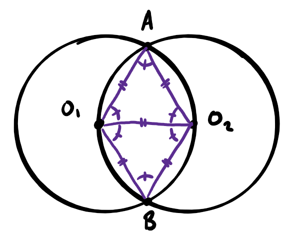
So we bear this in mind. I would consider proving that with the following figure.

There are number of ways to complete the argument. Here are a couple of more obscure ones that illustrate my approach.

Firstly, let’s ignore the result that and proceed directly to . It suffices to show that the blue angles are equal, which is equivalent to demonstrating that is cyclic.

To achieve this, we would like to show that the angle is equal to the red angle we’ve already discussed, and this follows by chasing round, using that is the centre of triangle ABC, and then the fact that is the external angle opposite in cyclic quadrilateral . Indeed, note that this use of an equal external angle rather than ‘opposite angle is 180 – […]’ is the textbook example of clear angle chasing, where focusing on equality rather than arithmetic massively cleans up many diagrams.

As a second, rather overblown way to complete the argument, let’s show that the angles at D and E are equal, without calculating them. Since are angle bisectors, we have two pairs of equal angles as shown.

It would suffice to show that these measures are themselves equal. This is saying that line is the external angle bisector of . And this is true, since is the arc-midpoint of AB on !

I hope these observations are interesting. But, to reiterate, this level of complexity is unnecessary, and arguments by congruent triangles or direct angle chasing are perfectly satisfactory too!

Problem Five

The punchline of this problem is that m(N) is an integer precisely if N is a triangle number, from which it is quick to count the number of such N.

But how to arrive that this punchline? It is reasonably clear that the N-set with minimal mean must have the form . One could proceed by setting up inequalities involving the means of and to establish a relationship between k and N.

But there is a more direct route. A useful, and very intuitive result about means is the following. If you have a set of numbers with mean x, and you add into the set a new number y, then the mean of the new larger set is between x and y. In particular, if y>x, then the new mean is larger than x.

In particular, consider the mean of . If it is less than k, then removing k gives a smaller mean. If it is greater than k+1, then adding k+1 gives a smaller mean. So since the mean is an integer, it must be equal to k or k+1. That is, we have

These lead to .

Problem Six

There must be some significance to the choice of 71 terms, and the 999,999 but it’s hopeless to try and see this immediately. In this scenario, it really is helpful to play around with semi-small examples.

Note that the second term is 1 regardless of whether we view this as P for PREVIOUS or S for SUM. However, if we then have an S, our sequence starts 1,1,2,2… or 1,1,2,4,… and these are bad, as once we have two even consecutive even numbers, we are doomed to see even numbers forever.

So once we have a common factor, that common factor is retained. How would we introduce a factor of, say, 11? Well, if you take 1,1,1,1,1,1,1,1,1,1,1 then take an S, you get 11, and afterwards you get either 11 or 22.

This gives a clue of the right way to set up the problem. For definiteness, we consider the second term to be an S. If you then consider a sequence of Ss and Ps, and write down the number of Ps between successive Ss (which may be zero) as a list , it holds that , and that each string of Ps introduces a factor of , leading to

Note that , so there exists a choice of the s that satisfies these relations simultaneously. (And if we had replaced 71 by a smaller choice, this would have been impossible.)

The actual answer to the problem is obtained by studying how to rearrange the blocks of SPPP…s, but the main challenge lies in reducing to this form.

I thought this was a hard problem for BMO, and was impressed to see some solutions under exam conditions.

Convex ordering on Galton-Watson trees

This blog was recently revived, via a post about convex ordering and its relevance to the problem of sampling with and without replacement that forms part of the potpourri of related results all sometimes referred to as Hoeffding’s inequality.

The previous post had been lying almost-complete but dormant for over two years. I revisited it because of a short but open-ended question about trees posed in our research group meeting by Serte Donderwinkel, one of our high-flying doctoral students.

Simplified Question:

For a Galton-Watson tree, can one obtain upper bounds in probability on the height of the tree, uniformly across all offspring distributions with mean ?

Note that in this setting, it is helpful to have in mind the classical notation for a Galton-Watson process, where typically , and is the sum of IID copies of the offspring distribution. Then we have

1) Subcritical case. When , we certainly have .

Furthermore, if we’re studying all such offspring distributions, this is the best possible upper bound, by considering the offspring distribution given by with probability and zero otherwise.

2) In the critical or supercritical case, it is possible that the height is infinite with probability one.

So neither case is especially interesting for now.

Refined question:

What if instead we aren’t trying to obtain a bound uniformly across all offspring distributions with given mean , but instead across a subset of these distributions? How do we determine which distribution in maximises the probability of reaching height k?

This is the question Serte was asking in our group meeting, in the setting where and the height k has a particular scaling. Also, as far as I understand, the approach outlined in this post didn’t provide strong enough bounds in this particular context. Happily, Serte has recently tied up all the corners of this project concerning the supercritical Galton-Watson forest, and interested readers can find her preprint here on the Arxiv.

Nonetheless the interpretation via convex ordering feels perfect for a blog post, rather than being lost forever.

Convex ordering for offspring distributions

The main observation is that given two offspring distributions X and Y, such that (which recall means that the means are the same but X is more concentrated) then a number of distributions associated to the Galton-Watson trees for X and Y also satisfy convex ordering relations.

As a warm-up, and because it was the original genesis, we first study heights. We will use the notation

to denote the two Galton-Watson processes. We shall compare and . If we write for the function defined on the non-negative integers such that

,

it holds that is convex. In particular, if , then , which exactly says that

We can then prove that by induction on . Note that is a convex function of n, regardless of the value of this probability, and so we have

By the induction hypothesis, this final quantity is at most

.

In conclusion, we have shown that holds for all k, and thus

To return to the original context, suppose we have a large class of offspring distributions and a subclass such that for all , there exists such that . Then one can obtain uniform bounds on the heights of Galton-Watson trees with offspring distributions drawn from by checking those generated from distributions in (which is particularly convenient if, for example, is finite).

Convex ordering of generation sizes

The above argument solves the original problem, but brushes over the natural question: is it true that ?

The answer is yes. Here’s a proof.

This follows from the following general statement:

Lemma 1: Suppose are non-negative valued RVs and the non-negative integer valued RVs also satisfy . Then

where are IID copies of X and, independently, are IID copies of Y.

Lemma 2: Suppose and , and the four random variables are independent. Then .

Proof of Lemma 2: First, note that for any random variable X, and convex function f

is a convex function of x.

(Indeed, this holds since “f(z+x) is convex” holds for every z, and any definition of convex will pass to the expectation.)

Now we can attack the lemma directly, we may write

But then for any , we know is convex, so , and it follows that

which proves the lemma.

Corollary 3: When are independent, and satisfy , then we have .

Proof of Lemma 1: Note that

follows from Corollary 3. So a useful question to consider is whether (*) is a convex function of n?

Denote this quantity by . To check convexity of a function defined on the integers, it suffices to verify that .

There is a canonical coupling between the RVs used to define all of , but it will be convenient to adjust the coupling, and write:

where is a further independent copy of . But note that for any choice and ,

(*)

(Essentially, this says that the ‘chord’ of f on the interval lies above the chord on interval or , which some people choose to call Karamata’s inequality, but I think is more helpful to think of as part of the visual definition of convexity.)

In any case, setting and taking expectations, we obtain

as required. So is convex. We may now finish off as

completing the proof of Lemma 1.

Final comments

• The analysis in this post is not sufficient to study the total population sizes of two Galton-Watson trees generated by X and Y. Note that in Lemma 2, it is important that the random variables are independent. Otherwise, we could, for example, consider with but clearly it should not hold that . So for total population size, since are not independent, an alternative approach would be required.
• A further characterisation of convex ordering is given by Strassen’s theorem [Str65], which is touched on in the previous post, and to which I may return to in a future post on this topic. This may be a more promising avenue for established a convex ordering result on total population size.
• Lemma 1 requires that X,Y are non-negative. Note that during the argument we set , and when we relax the non-negative support condition, it is no longer guaranteed that , which is crucial for the step which follows.
• In a recent article in ECP addressing Lemma 1 by a different method, Berard and Juillet [BJ20] provide a simple example showing that the non-negative assumption is genuinely necessary. Consider the random variable with equal probability so . But then, taking both X and Y to be simple random walk on , we do not have .

References

[BJ20] – Berard, Juillet – A coupling proof of convex ordering for compound distributions, 2020

[Str65] – Strassen – The existence of probability measures with given marginals, 1965

Hoeffding’s inequality and convex ordering

A number of previous posts on this blog have discussed Markov’s inequality, and the control one can obtain on a distribution by applying this to functions of the distribution, or functions of random variables with this distribution. In particular, studying the square of the deviation from the mean leads to Chebyshev’s inequality, while even stronger bounds can sometimes be obtained using , for some appropriate value of . Sometimes this final method, which relies on the finiteness of is referred to as a Chernoff bound, especially when an attempt is made to choose the optimal value of t for the estimate under consideration.

The case of a random walk, that is the sum of IID increments, is particularly well-studied. In [Ho63], Hoeffding studies a generalisation where the increments are merely independent, and outlines a further generalisation to discrete-time martingales, which is developed by Azuma in [Az67], leading to the famous Azuma-Hoeffding inequality. A key feature of this theorem is that we require bounded increments, which leads to tight choices of in the Chernoff bound for each increment.

In addition, [Ho63] addresses the alternative model where the increments of a random walk are chosen uniformly without replacement from a particular set. The potted summary is that the sum of random increments chosen without replacement has the same mean, but is more concentrated that the corresponding sum of random increments chosen with replacement. This means that any of the concentration results proved in the earlier sections of [Ho63] for the latter situation apply equally to the setting without replacement.

Various versions of this result are referred to as Hoeffding’s inequality by the literature, and the main goal of this short article is to list some results which are definitely true about this setting!

(Note, in some contexts, ‘Hoeffding’s inequality’ will mean the concentration bound for either the with-replacement or the without-replacement setting. In this blog post, we are discussing inequalities comparing these two settings.)

Starting point – second moments in ‘vanilla’ Hoeffding

We won’t use this notation heavily, but for now let’s assume that we are studying a (multi)set of values , and will study a sequence of m elements from this set with replacement (ie chosen in an IID fashion), and a sequence of m elements chosen from this set without replacement.

Some preliminary remarks:

• The s are still chosen uniformly which can be interpreted as
  • Any permutation of the multiset is equally likely to appear as ;
  • If determining the sequence one element at a time, then in a conditional sense, the choice of the ‘next’ element is uniform among those elements which have not yet been chosen.
• In particular, the sequence is exchangeable (though not knowing what that means will not be a significant impediment to what follows).
• It is clear that , so concentration around this common mean is the next question of interest.
• Intuitively, when , we wouldn’t expect there to be much difference between sampling with or without replacement.
• When sampling without replacement, the cases m and N-m are symmetric with respect to the sum of and, in particular, have the same concentration.

As a brief warmup, we establish that

Note that the RHS is , where is the variance of a single uniform sample from . Since these sums have the same mean, it suffices to show that

But this really has nothing to do with probability now, since these quantities are just symmetric polynomials in . That said, we gain a little bit if we use the exchangeability property to rewrite the LHS and the RHS as

Since , it remains to handle the cross term, which involves showing that

which really is an algebra exercise, and can be demonstrated by the rearrangement inequality, or Chebyshev’s inequality (the other one – ie sequence-valued FKG not the probabilistic second-moment bound one), or by clever pre-multiplying and cancelling to reduce to Cauchy-Schwarz.

In [BPS18], which we will turn to in much greater detail shortly, the authors assert in the first sentence that Hoeffding treats also the setting of weighted sums, that is a comparison of

A casual reader of [Ho63] may struggle initially to identify that this has indeed happened. At the level of second-moment comparison though, the argument given above carries over essentially immediately. We have

and of course the corresponding decomposition for , from which the variance comparison inequality follows as before.

Convex ordering

For many applications, variance is sufficient as a measure of concentration, but one can say more. As a prelude, note that one characterisation of stochastic ordering (which I have sometimes referred to as stochastic domination on this blog) is that

whenever f is a non-decreasing function. Unsurprisingly, it’s the direction which is harder to prove, though often the direction is the most useful in applications.

[To inform what follows, I used a number of references, in particular [BM05].]

A natural extension to handle concentration is (stochastic) convex ordering, which is defined as

whenever f is a convex function. Note immediately that this definition can only ever apply to random variables for which . Otherwise, consider the functions , both of which are convex.

This sort of comparison has plenty of application in economics and actuarial fields, where there is a notion of risk-aversion, and convexity is the usual criterion to define risk (in the sense that the danger of a significant loss is viewed as more significant than a corresponding possibility of a significant gain). Also note that in this context, X is preferred to Y by a risk-averse observer.

In fact, it can be shown [Oh69] that a sufficient condition for is the existence of such that

where is the usual distribution function of X. That is, the distribution functions ‘cross exactly once’. Note that in general .

We will return later to the question of adapting this measure to handle distributions with different expectations, but for now, we will return to the setting of sampling with and without replacement and show that

This is the result shown by Hoeffding, but by a more complicated method. We use the observations of [BPS18] which are stated in a more complicated setting which we may return to later. For notational convenience, let’s assume the elements of are distinct so that ‘repetitions of ‘ has an unambiguous meaning.

We set up a natural coupling of as follows. Let be IID uniform samples from , and generate by removing any repetitions from .

Note then that given the sequence , the multiset of values definitely includes at least once, but otherwise includes each either zero, one or more times, in a complicated way. However, this distribution doesn’t depend on the values taken by , since it is based on uniform sampling. In particular, if we condition instead on the set , we find that

and so we may coarsen the conditioning to obtain

This so-called martingale coupling is very useful for proving convex ordering. You can think of as saying “X is generated by Y plus additional randomness”, which is consistent with the notion that Y is more concentrated than X. In any case, it meshes well with Jensen’s inequality, since if f is convex, we obtain

So we have shown that sampling without replacement is greater than sampling with replacement in the convex ordering, if we consider sums of the samples.

If we want to handle weighted sums, and tried to reproduce the previous argument directly, it would fail, since

which is not in general equal to .

Non-uniform weighted sampling

Of course, it’s not always the case that we want to sample according to the uniform distribution. My recent personal motivation for investigating this setup has been the notion of exploring a graph generated by the configuration model, for which vertices appear for the first time in a random order that is size-biased by their degrees.

In general we can think of each element of as having some weight w(i), and at each step, we pick from the remaining elements with probability proportion to w(i). This procedure is known in other contexts as successive sampling. Note that the sequence is no longer exchangeable. This is clear enough when there are two elements in , and . So it is much more likely that than .

In addition, it will in general not be the case that

and this is easily seen again in the above example, where while .

However, one can still compare such distributions, with the notion of increasing convex ordering, which is defined as:

for all convex non-decreasing functions f. From an economic point view, increasing convex ordering becomes a comment on the relative contribution of losses above some threshold between the two distributions (and that X is better or worse than Y for all such thresholds), and is sometimes called stop-loss order. More formally, as in [BM05] we have:

In [BPS18], the authors study the case of successive sampling where the weights are monotone-increasing in the values, that is , of which size-biased sampling is a special case. With this setup, the heuristic is that ‘large values are more likely to appear earlier’ in the sample without replacement, and making this notion precise underpins all the work.

The coupling introduced above is particularly useful in this more exotic setting. The authors show that conditional on the event A of the form , one has

This is achieved by comparing the explicit probabilities of pairs of orderings for with exchanged. See [BPS18] for this short calculation – a link to the Arxiv version is in the references. So to calculate , we have the setup for the rearrangement inequality / Chebyshev again, as

As before, letting be the sums of the samples with and without replacement, respectively, we have , which the authors term a submartingale coupling. In particular, the argument

works exactly as before to establish convex ordering.

References

[Az67] – Azuma – 1967 – Weighted sums of certain dependent random variables

[BM05] – Bauerle, Muller – 2005 – Stochastic orders and risk measures: consistency and bounds. (Online version here)

[BPS18] – Ben Hamou, Peres, Salez – 2018 – Weighted sampling without replacement (ArXiv version here)

[Ho63] – Hoeffding – 1963 – Probability inequalities for sums of bounded random variables

[Oh69] – Ohlin – 1969 – On a class of measures of dispersion with application to optimal reinsurance

BMO1 2019

The first round of the British Mathematical Olympiad was sat yesterday. The paper can be found here, and video solutions here. Copyright for the questions is held by BMOS. They are reproduced here with permission.

I hope any students who sat the paper enjoyed at least some of the questions, and found it challenging! The following brief commentaries on the first three problems are not official solutions, and are not always full solutions at all, but contain significant steps of solutions, so would be best saved until after you have attempted the problems, if you are planning to do so.

Question 1

Show that there are at least three prime numbers p less than 200 for which p+2, p+6, p+8, p+12 are all prime. Show also that there is only one prime number q for which q+2, q+6, q+8, q+12, and q+14 are all prime.

It is a major open problem of considerable interest in mathematics to study primes p for which p+2 is also a prime. You are warmly encouraged to have a look at the video of this talk by oucolleague Vicky Neale which discusses this topic in an accessible fashion.

Fortunately, the statement of the second half of this BMO1 problem is not open, but the wider context is a sign that we should be looking for a simple reason why the numbers {q, q+2, q+6, q+8, q+12, q+14} cannot all be prime very often. A candidate for a simple reason is that one of them must be divisible by eg 6 (since there are six numbers), but of course this is not true, eg when q=3, or any other odd value. However, it is the case that one of these numbers must be divisible by 5. You could show this in a few ways:

• studying what the last digit could be (a number is divisible by 5 precisely when it’s final digit is 0 or 5);
• studying the remainder of each of the numbers under division by 5;
• these are in fact pretty much the same thing, only the first option cycles with period ten, whereas the second cycles with period five.

In particular, the only chance that this collection consists of six prime numbers is when one of them is 5, since this is the only multiple of 5 which is a prime! So we need to check q=3, and q=5, and the latter leads to a solution, while q=3 does not, since q+6=9 is not prime.

In fact, the question is true even if we remove one of the terms {q+2, q+6, q+8, q+12, q+14} from consideration. To check that you understand the argument, see if you can work out which term(s) could be removed without breaking the solution?

For the first part, you will probably need to write down some integers less than 200 and check which are and aren’t prime, and maybe you have some shortcuts to narrow down the pool of candidates for p, but this doesn’t have to appear on your final solution. It really is enough to write down your three proposals for p, perhaps indicating what {p, p+2, p+6, p+8, p+12} are in these cases as a sanity check!

Question 2

A sequence of integers satisfies the relation:

(*)

for all positive integers n. What are the possible values of ?

We can ‘solve’ the equation (*) by viewing it as a quadratic in the variable , with coefficients involving . We end up showing that

(**)

Note that this is a problem if is even, since neither of these possibilities for the value of is actually an integer. So certainly cannot be even, since then we can’t even construct a sequence of length 2, let alone an infinite sequence!

Crucially, one of the options in (**) is odd, and one of the options is even. It’s helpful to think of trying to construct the sequence one term at a time starting from , where at each step we must ‘pick the odd option next’ as otherwise we’d be stuck at an even number, and couldn’t extend the sequence.

The exact wording for how you write this argument isn’t essential. What’s important is that you are clear about what you are trying to assert. Hopefully you are trying to assert something like:

For every odd choice of , there does exist an (infinite) sequence satisfying (*).

Why is this true? Because you can construct the sequence one term at a time. It’s not really necessary to set this up as a formal induction. Rather, you just need to tell the reader that you know how to ensure you never get stuck, namely by always choosing the odd option for , so that you do indeed end up with an infinite sequence.

Question 3

Two circles are tangent at P. A common tangent, not through P, touches at A, and at B. Points C and D, on respectively, are outside triangle APB, such that P lies on line CD.

Prove that AC is perpendicular to BD.

Here’s a diagram for this problem, lifted from the video. Cropped Dominic is pointing out where AC and BD meet, which I’ve chosen to call X.

As so often in olympiad problems, especially in geometry, the key to success is choosing the right characterisation of the property you are required to prove. In this case, proving that the angle at X is a right angle is awkward via a direct calculation since we don’t really know anything about X except its literal definition. However, an alternative is to show that the angles at C and at D sum up to 90. This is a much better contender for a useful characterisation since we know a lot more about C and D.

For example, C and D both lie on a circle, so are eligible for using circle theorems. Since we have several tangents, the alternate segment theorem might well be useful here. Indeed, if can apply it twice for each of C and D, and in doing so, characterise all the angles of triangle APB in terms of the angles at C and D:

There’s no harm in being informal at this stage. Within triangle APB, we know that the sum of two copies of the red angle and two copies of the black angle is 180 degrees, and so we can read off that the sum of the angles at C and at D is 90 degrees.

For the video presentation, I added the common tangent at P, which did turn out to be useful, and the centres and radii of the circles, which didn’t turn out to be useful. It’s generally a good idea to be thoughtful and flexible about what to include on a diagram. You can probably imagine why it might have been a distraction if we’d had lots of extra lines like BC or PX added on the figure, without any evidence they would be useful to the solution.