Finitely many solutions

This post is aimed at secondary-school students pitched roughly at the level of the British Mathematical Olympiad. It is ostensibly about a certain class of number theory problems, but the main underlying mathematical principle is broader than this. The post is based on an in-person session I have given to students and at teachers’ conferences a few times over the past five years, but I’ve chosen to write it up at this moment because of the connection to Problem 4 on the most recent BMO1 paper, which we discuss later in the post.

Prologue

Alice and Bob make the following statements:

• Alice: all prime numbers are odd.
• Bob: we can’t say anything about whether prime numbers are odd or even.

These are different types of statement, one objective, one more subjective; but both are wrong. Alice is wrong because 2 is a prime, and 2 is of course even. Bob is wrong because while Alice is wrong, and the alternative statement “all prime numbers are even” is even more wrong¹, there are plenty of possible statements that are true and useful, including

• Cleo: all prime numbers are odd except 2.

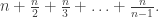
and weaker versions (that may be more relevant in other contexts) like “all primes greater than are odd”.

The characters now turn their attention to another family of integers, the square numbers , and the sixth powers

• Alice: no square numbers are prime.
• Bob: I agree.
• Alice: most square numbers are not sixth powers.
• Bob: hang on, but infinitely many square numbers are sixth powers?

The difficulty in the second statement is what does most mean in this context? The square of an integer n is a sixth power if and only if n is a cube, and so Alice’s statement is equivalent to the statement “most positive integers are not cubes”, which is intuitively reasonable, but would require more clarification than the analogous statement “most primes are odd”. Is it not relevant, for example, that 1/4 of the first eight positive integers are in fact cubes?

It is not impossible to formalise this notion of most in a reasonable way to permit the two statements above².

But the bulk of this post will discuss situations that extend the first of these conversations, ie when it’s not true to say “all element of X have property Y”, but where it’s nonetheless possible to make a useful intermediate statement.

Warmup problems

I hope most readers know how to solve an equation such as

and indeed learning how to solve such equations forms a important milestone in mathematical education as the first example of various principles of algebra. When such equations are still novel, teachers would be advised to avoid examples such as

for which the answers are, respectively, ‘no solutions’ and ‘every x satisfies this’. While they are perfectly valid equations, it means something slightly different to solve them, since the answer set has different structure and, more importantly, the method is different since it doesn’t consist of a sequence of a manipulations leading directly to the required conclusion .

However, I mention this in passing to clarify that even in the simplest possible family of equations (probably encountered somewhere between ages 9 and 13) we are mindful that not all equations have unique solutions.

I’ve adapted a problem from the American competition AIME:

Find all integers such that is a prime.

One could start by writing if you wish, but in fact we only need to work with the left hand side, so it’s better to avoid this if possible. The key to this problem is to avoid the prime condition initially, and just manipulate the LHS until it simplifies as

(*)

which is never a prime, since is a square number and so, as already discussed, never a prime.

So at a meta-level, comparing with the other problem in this section, this one also begins with reversible algebraic manipulations, but does not end with a direct reduction to , and indeed the final step is not reversible at all.

Finally, we remark that the original version of the AIME problem was

Prove that for all integers , is a perfect square.

The same algebraic reduction as (*) resolves the original version without an extra step concerning primes.

To be, or not to be, a perfect square

The rest of this article will focus entirely on problems of the form: find all positive integers n such that […] is a perfect square.

As setup, we’ll always consider a function f(n), and the sequence f(1),f(2),f(3),… and the question, comment on the set of n is f(n) a square? In particular, this is a more open-ended question than for which n is f(n) a square, which requires a more exact answer. We’ll aim for one of the following possible answers:

• f(n) is always a square;
• f(n) is a square for infinitely many n;
• f(n) is a square for only finitely many n;
• f(n) is never a square.

Clearly this is not an exhaustive list of possible descriptions³ of the set under discussion, but it will do for now. The difference between the second and the third bullet point can be thought of as: “are there arbitrarily large values of n for which f(n) is a square?”

As some examples:

• is always a square, because is always a square.
• is never a square, because the only squares that differ by 1 are {0,1} which aren’t attainable when .
• is a square for only finitely many n, because the only squares that differ by 3 are {1,4}.

Exercises to try yourself

• ,
• or, now with p ranging over the set of prime numbers: .

Some discussion of some of these follows later to avoid spoilers.

BMO1 2023, Problem 4

This problem does not have exactly the same structure as the previous exercise. A solution will follow shortly, but before starting, [spoilers] I want to emphasise that the main part of the solution involves framing this problem exactly as in the exercise above.

• We will establish that there are only finitely many n such that is a square, using a classical number theory argument.
• In doing so, we will eliminate all integers n that are at least some threshold value K from consideration (which we think of as “n large”, even though in this case it isn’t so large).
• The actual set of solutions comes from check the remaining “small” values of n.
• The point to emphasise is that while this third bullet is definitely an important component of a successful solution (and does feel closest to actually addressing the “find all” aspect of the problem statement), it is not really the key step, since checking a small number of possibilities is fundamentally much more straightforward than an argument to eliminate the other infinitely-many integers.

This overall structure is very common when solving Diophantine equations involving integers, even if the exact statement isn’t “find all n such that […] is a perfect square”.

Anyway, to the solution of this problem. As in many problems of this difficulty in this number theory, it’s really useful to aim to factorise and analyse the factors, remembering that they are integers! In this case, writing doesn’t suggest an easy factorisation of the LHS, but rewriting as does now have a nice factorisation, using difference of two squares on the RHS:

Here the two factors are (k-1) and (k+1). We know nothing about k, so we know nothing intrinsic about these factors, except that they differ by 2. But now when we consider that their product is , we can start to make some serious deductions⁴.

• (k-1) and (k+1) differ by two, and so have the same parity⁵. Then is even, and so in fact both factors are even.
• But more than this, one factor will be a multiple of 4, while the other will not be. So all the powers of 2 within (which may include additional factors of 2 coming from n) apart from one, must be included in one of the factors.
• The idea is that is generally much larger than n, and so this will force one of the factors to be much larger than the other factor, which is not permitted. (Recall that the factors differ by 2.)

So formally, we might write that and . These are inequalities not equalities because some of the factors of n could be in (k+1) not (k-1) and/or a priori, we could have and etc. This leads to

(*)

and we now have exactly the language to describe the truth of this inequality! It is only true for finitely many positive integers n. There are a number of ways to prove this, but it is important that we do provide a lower bound. One possibility is to check that (*) holds for n=5, and then prove (*) for all by an inductive argument.

At this point, we have shown that is not a perfect square for , and so at this point it really is easiest just to check by hand, which reveals that work.

To link this to the background, note that this final procedure of “finding all the solutions” really had nothing in common structure-wise with “solving “, for which substituting in various values of x would never constitute part of a good solution.

Comments on exercises

• is a square for infinitely many n, while is never a square, for reasons that are often framed in the language of quadratic residues.
• is a square for infinitely many n (specifically, when n is even), while is a square only when n=3, which can be seen via a similar argument to the argument above for the BMO problem. Meanwhile is never a square, which can also be checked using quadratic residues.
• is a square for infinitely many n (specifically, when ), while is a square for only one prime p, since only one prime is divisible by 3.
• is only a square for finitely many n, because when n is large, we have . This style of argument is sometimes called square-sandwiching, although it can of course be deployed in contexts other than squares. Problems that turn on this method have appeared in BMO surprisingly often in the past 15 years. For this particular example, note that one does have to check a handful of values to confirm it is for finitely many but at least one n (rather than for no n).

Footnotes

1. of course, writing even more wrong is in itself making a nuanced comment about the parity of the prime numbers. ↩︎
2. given a set , a natural formalisation of the notion that ‘most integers are not in A’ would be that In other words, the proportion of elements of A amongst the first n integers vanishes as . This is certainly true when A is the set of cubes.
   There are many sets for which this limit does not exist, including quite natural sets like the integers whose decimal representation starts with a 1, and so a full treatment of this notion of asymptotic density would require more than a footnote. ↩︎
3. in particular, we might wish to draw a distinction between f(n) is a square for infinitely many n and the stronger statement f(n) is a square for all-but-finitely many n, and in some applications that difference is crucial. ↩︎
4. A common error is to make some reasonable-sounding assumption about how the factors of are split between (k-1) and (k+1), for example by assuming that and because this is visually a natural way to pair them up. ↩︎
5. parity refers to whether a number is odd or even. ↩︎

Symmedians and Balkan MO 2017 Q2

While I was away, I wrote about my latest approach to teaching geometry at olympiad camps. This post will end up being about Q2 from the Balkan MO which took place yesterday in Macedonia, but first there is quite a long prelude. My solution, and probably many solutions, to this problem made use of a standard configuration in triangle geometry, namely the symmedian. I want to introduce the configuration, give some simpler examples in practice, and along the way talk about my slightly patched-together philosophy about the merits of practising Euclidean geometry.

The symmedian

Draw a triangle ABC, with A at the top of the page, and extend the rays AB and AC. The median is the line from A through M, the midpoint of BC. Now take points D and E on AB and AC respectively. The following properties are equivalent:

• DE is parallel to BC;
• triangle ADE is similar to triangle ABC;
• the median of ABC passes through the midpoint of DE, and thus is also the median of ADE.

I think it’s a little awkward to prove either of the first two from the third – ratios of areas works – but the rest of the equivalences are straightforward. Later I’m going to talk about the difference between an exercise and a problem. These are all, at best, exercises.

Now take B’ on the ray AC, and C’ on the ray AB such that triangle AB’C’ is similar to triangle ABC. One way to achieve this is to take B’ and C’ to be the reflections in the angle bisector of A of B and C respectively (so then AB’=AB and AC’=AC). We say the line B’C’ is antiparallel to BC, as is any other line DE parallel to B’C’. (Probably this should say ‘with respect to triangle ABC’ or similar, but the context here is very clear, and I want this to seem natural rather than opaque.) Note that DE is an antiparallel line iff BCED is a cyclic quadrilateral. We should remember that, as cyclic quadrilaterals are the signposts for progress in both exercises and problems.

The median of triangle AB’C’ obeys the same equivalences as described above, and so bisects any antiparallel segment. We call the median of triangle AB’C’ the symmedian of triangle ABC. Using the first set of equivalences, the symmedian of triangle ABC bisects any line antiparallel to BC. Furthermore, by construction, the symmedian is the image of the median of ABC under reflection in the bisector of the angle at A. We sometimes say that the symmedian is the isogonal conjugate of the median.

That’s my definition. Note that there was essentially one definition then a couple of easy equivalent definitions. At no point again will I discuss the equivalence of these definitions – we have to take that for granted if we want to get on to more interesting things.

Intersection of tangents + concurrency

Now, in triangle ABC, draw the tangents to the circumcircle at B and C. These meet at P. It turns out that AP is the symmedian. This could have been our definition of a symmedian, but it wasn’t, so let’s quickly prove this.

Trigonometric arguments are very accessible, but I’ll give a Euclidean argument. Draw the antiparallel DE through P, as shown. Our task is to show that EP=PD. At this point, I would again say that this is an exercise.

We colour the angle ABC in green. Two angles around point C share this measure by the alternate segment theorem. The angle at E shares this measure because DE is antiparallel. Therefore CPE is isosceles, and so EP=CP. But CP=BP, so by applying the same argument for the orange angles, we get EP=CP=BP=DP as required.

Pause to regroup. Proving this wasn’t hard, but it was perhaps surprising. If this was all new to you, and I told you to consider the reflection of the median in the angle bisector, you probably wouldn’t instantly exclaim “it goes through the tangent intersection!” So this is a useful piece of knowledge to have gained, in case we ever have to work with the intersection of two tangents like this. Maybe it won’t be useful, but maybe it will. Maybe the statement itself won’t but some extra insights from the proof will be useful, like the fact that we actually showed P is the centre of the circle BCED, and thus angles ECD=EBD=90.

A second property is that in a triangle ABC, the symmedian from A, the symmedian from B and the symmedian from C intersection at, naturally, the symmedian point, which is usually denoted K. This comes from the fact that each symmedian is the isogonal conjugate of the respective median, and the medians are known to concur at the centroid. I’m not going to get into this now.

Configurations – an example

Here’s a problem. Take an isosceles trapezium ABCD as shown (ie throughout I don’t want to worry about alternative diagrams).

Let M be the midpoint of AD, and let E be the point on CM such that angle DBM = EBA. Prove that ABCDE is cyclic.

Well, certainly ABCD is cyclic. So we just need to show E also lies on that circle. And we have two equal angles, but they aren’t in the right place to conclude this immediately. However, we have angle MCA = DBM = EBA, so ABCE is cyclic, and the result follows.

Why is angle MCA = DBM? Well, the isosceles trapezium has an axis of (reflective) symmetry, and MCA is the is image of DBM under that reflection. Simple. If we wanted to do it with congruent triangles, this would all be a bit more laborious. First have to show BD=AC using one set of congruent triangles, then CM=BM using another, finally finishing using DM=MA. This is much less interesting. The symmetry of the configuration is a higher-level observation which could be proved from the axioms of geometry if necessary, but gives us more information more quickly. When we use a configuration like the symmedian configuration, we are really doing a higher-again-level version of this.

Anyway, that problem is fine, but it’s not especially difficult.

Consider instead the following problem. (I saw this online, possibly with slightly different notation, a few days ago and can no longer find the link. If anyone can help, I will add the link.)

Let AB be a chord of a circle, with midpoint M, and let the tangents at A and B meet at P. Consider a line through P which meets the circle at C and D in that order. Extend CM to meet the circle again at E. Show DME is isosceles.

Here’s a diagram, though it includes some clues.

I thought this was a fun problem, and for a while I couldn’t do it because despite lots of equal angles and equal lengths, I couldn’t conjure any congruent triangles in the right places, and I didn’t care enough about solving it to get involved in trigonometry. Then came the moment of insight. We have a midpoint, and also the intersection of the tangents. So DP is the symmedian of triangle DAB, and DM is the median. This gives us the two equal orange angles. Cyclicity gives us an extra equal angle at E as well.

Note now that the situation is very very similar to the previous question (after changing some of the labels), only this time we know ACBDE is cyclic, but don’t know that ABDE is an isosceles trapezium. If ABDE is an isosceles trapezium, we are clearly finished, as then by the same symmetry argument, EM=DM. This direction is probably harder to prove than the direction of the previous problem. Again there are a couple of ways to proceed, but one way is to consider the point E’ such that ABDE’ is an isosceles trapezium, and arguing that E’ lies on the given circle, and the circle through BME, and thus must coincide with E, in a reverse reconstruction argument.

Anyway, this is all slightly a matter of taste, but I would say the second problem is much much more fun than the first problem, even though the second part of the solution is basically the first problem but in a more awkward direction. If you’re going to do Euclidean geometry at all (very much another question), I think you should do questions like the second question wherever possible. And the enjoyable ‘aha moment’ came from knowing about the symmedian configuration. Is it really plausible that you’d look at the original diagram (without the dashed orange lines) and think of the antiparallel to AB in triangle DAB through point P? Probably not. So knowing about the configuration gave access to the good bit of a nice problem.

‘Philosophy of this sort of thing’

If the goal was to solve the second problem in a competition, knowing about the symmedian configuration would be a big advantage. I’ve tried to justify a related alternative view that knowing about the configuration gave access to an enjoyable problem. The question is how many configurations to study, and how hard to study them?

We tend not to think of cyclic quadrilaterals as a special configuration, but that is what they are. We derived circle theorems from the definition of a circle so that we don’t always have to mark on the centre, every single time we have a cyclic quadrilateral. So becoming familiar with a few more is not unreasonable. In particular, there are times when proofs are more important than statements. In research (certainly mine), understanding how various proofs work is the most important aspect, for when you try to extend them or specialise. And in lots of competition problems, the interesting bit is normally finding the argument rather than basking in wonder at the statement (though sometimes the latter is true too!).

To digress briefly. In bridge, I don’t know enough non-obvious motifs in bidding or gameplay to play interesting hands well. I trust that if I thought about some of it very very carefully, I could come up with some of them, especially in gameplay, but not in real time. And it is supposed to be fun right?! Concentrating very very hard to achieve a basic level of competence is not so enjoyable, especially if it’s supposed to be a break from regular work. The end result of this is that I don’t play bridge, which is a shame, because I think the hurdles between where I am currently and a state where I enjoy playing bridge are quite low. If I knew I was going to play bridge regularly, a bit of time reading about conventions would be time well spent. And obviously this applies equally in pursuits which aren’t directly intellectual. Occasionally practising specific skills in isolation broadens overall enjoyment in sport, music, and probably everything. As anyone who’s played in an orchestra knows, there are standard patterns that come up all the time. If you practise these occasionally, you get to a stage where you don’t really need to concentrate that hard in the final movement of Beethoven 5, and instead can listen to the horns, make funny faces at the first violins, and save your mental energy for the handful of non-standard tricky bits. And of course, then move on to more demanding repertoire, where maybe the violas actually get a tune.

This is highly subjective, but my view is that in all these examples are broadly similar to configurations in geometry, and in all of them a little goes a long way.

How? In lots of the geometry configurations you might meet in, for example, a short session at a training camp, most of the conclusions about the configurations have proofs which, like in our symmedian case, are simple exercises. Once you’ve got over some low initial experience hurdles, you have to trust that you can normally solve any simple exercise if required. If you can’t, moving on and returning later, or asking for help is a good policy. The proof shown above that symmedians pass through tangent meet points (and especially a trigonometric alternative) really isn’t interesting enough to spend hours trying to find it. The statements themselves are more useful and interesting here. And it can often be summarised quite quickly: “symmedians are the isogonal conjugates of the medians, so they bisect antiparallels, meet at K, and pass through the alternate tangent meeting points.” Probably having a picture in your mind is even simpler.

There’s a separate question of whether this is worthwhile. I think solving geometry problems occasionally is quite fun, so I guess yes I do think it is worthwhile, but I understand others might not. And if you want to win maths competitions, in the current framework you have to solve geometry problems under time pressure. But from an educational point of view, even though the statements themselves have no real modern research value, I think a) that’s quite a high bar to set, and there’s no a priori reason why they should – >99.9% of things anyone encounters before university have no value to modern research maths; b) in terms of knowledge acquisition, it’s similar in spirit to lots of things that are relevant to later study. I don’t have to solve PDEs very often, but when I do, I hope they are equivalent or similar to one of the small collection of PDEs I do know how to solve. If I worked more with PDEs, the size of this collection would grow naturally, after some initial struggles, and might eventually match my collection of techniques for showing scaling limits of random processes, which is something I need to use often, so the collection is much larger. Maybe that similarity isn’t enough justification by itself, but I think it does mean it can’t be written off as educationally valueless.

Balkan MO 2017 Question Two

An acute angled triangle ABC is given, with AB<AC, and is its circumcircle. The tangents at B,C respectively meet at L. The line through B parallel to AC meets at D. The line through C parallel to AB meets at E. The circumcircle of triangle BCD meets AC internally at T. The circumcircle of triangle BCE meets AB extended at S. Prove that ST, BC and AL are concurrent.

Ok, so why have I already written 1500 words about symmedians as a prelude to this problem? Because AL is a symmedian. This was my first observation. This observation is then a route into non-Euclidean solutions. It means, for example, that you can describe the point of concurrency fairly explicitly with reference to triangle ABC. If you wish, you can then proceed using areal coordinates. One member of the UK team, whom I know is perfectly capable of finding a synthetic solution, did this. And why not? It’s a competition, and if you can see a method that will definitely work, and definitely take 45 minutes (or whatever) then that’s good.

I was taking a break from work in my office, and had no interest in spending the time evaluating determinants because that isn’t enjoyable at any level, so I focused on the geometry.

I think there’s a good moral from the diagram above, which is the first moderately correct one I drew. I often emphasise that drawing an accurate diagram is important, as it increases the chance that you’ll spot key properties. In this case though, where you’re trying to examine a known configuration, I think it’s more important what you choose to include on your diagram, than how accurately you draw it. (In a moment, we’ll see why it definitely wasn’t very accurate.)

In particular, what’s not on the diagram? E is not on the diagram, and S got added later (as did the equal length signs in TB and CS, which rather spoil what’s about to happen). My first diagram was wildly incorrect, but it also suggested to me that the line ST was hard to characterise, and that I should start by deducing as much as possible about S and T by themselves. So by symmetry, probably it was enough just to deduce as much as possible about T.

Label the angles of triangle ABC as <A, <B, And therefore TB is an antiparallel in triangle ABC. (Note this doesn’t look antiparallel on my diagram at all, but as I said, this didn’t really matter.) Obviously you then guess that CS is also an antiparallel, and on a different diagram I checked this, for essentially the same reasons.

We haven’t yet made any use of the symmedian, but this is clearly where it’ll be useful. Note that if we didn’t know about everything in the prelude, we might well have deduced all of this, but we might not have thought to prove that AL bisects TB unless we’d drawn a very accurate diagram.

At this point, we have to trust that we have enough information to delete most of the diagram, leaving just {A,B,C,S,T} and the line AL. There are a few ways to finish, including similar triangles if you try very hard or trigonometry if you do it right, but again knowledge of some standard configurations is useful. Probably the quickest way is to use Ceva’s theorem in triangle ACS. You can also use Menelaus’ theorem in ABC, so long as you know a little bit about where the symmedian meets the opposite side.

An alternative is the following. We have a complete quadrilateral here, namely BTCS, and the intersection of all its diagonals. One is A, one is the proposed point of concurrency, and one is the point at infinity, since TB || CS. You can chase that, but I found it more clear to let P be the intersection of ST and BC (which we want to prove lies on AL), then look at the complete quadrilateral ATPB. Then AT and BP meet at C, and AB and TP meet at S. So if we look at where the diagonals of ATPB meet the line CS, we have a harmonic range.

If I’d wanted, I could instead have written the prelude about harmonic ranges, but I had fewer ideas how to set these up in a slick Euclidean way. Also, it feels better to talk about the start, rather than the end of a proof, especially when there were alternative endings. Anyway, a harmonic range is a collection of two pairs of points on a line (A, B; C, D), satisfying the following ratio of directed lengths:

A classic example is when D is the point at infinity, the RHS is -1, and so C is the midpoint of AB. Being happy about using the point at infinity is a property of projective geometry, of which this is a good first example. Anyway, returning to the problem, we are looking at where the diagonals of ATPB meet line CS, and this pair of points forms a harmonic range with (C,S). TB meets CS at the point at infinity, and so AP meets CS at the midpoint of CS. But from the symmedian configuration, AL bisects CS, so AP and AL are in fact the same line, and so P lies on AL as required.

I think was a brilliant example of when knowing a bit of theory is enjoyable. It wasn’t at all obvious initially how to use the symmedian property, but then the observation that TB is antiparallel felt like a satisfying breakthrough, but didn’t immediately kill the problem.

The Envelope ‘Paradox’

At the recent IMO in Hong Kong, there were several moments where the deputy leaders had to hang around, and I spent some of these moments discussing the following problem with Stephen Mackereth, my counterpart from New Zealand. He’s a mathematically-trained philosopher, so has a similar level of skepticism to me, but for different reasons, regarding supposed paradoxes in probability. Because, as we will see shortly, I don’t think this is a paradox in even the slightest fashion, I think there’s probably too much written about this on the internet already. So I’m aware that contributing further to this oeuvre is hypocritical, but we did the thinking in HKUST’s apparently famous Einstein Cafe, so it makes sense to write down the thoughts.

[And then forget about it for eight weeks. Oops.]

The ‘Paradox’

Here’s the situation. A cryptic friend gives you an envelope containing some sum of money, and shows you a second envelope. They then inform you that one of the envelopes contains twice as much money as the other. It’s implicit in this that the choice of which is which is uniform. You have the option to switch envelopes. Should you?

The supposed paradox arises by considering the amount in your envelope, say X. In the absence of further information, it is equally likely that the other envelope contains X/2 as 2X. Therefore, the average value of the other envelope is

So you should switch, since on average you gain money. But this is paradoxical, since the assignment of larger and smaller sums was uniform, so switching envelope should make no difference.

Probabilistic setup

This is not supposed to be a problem on a first-year probability exercise sheet. It’s supposed to be conducive to light discussion. So saying “I won’t engage with this problem until you tell me what the probability space is” doesn’t go down terribly well. But it is important to work out what is random, and what isn’t.

There are two sources of randomness, or at least ignorance. Firstly, there is the pair of values contained in the envelopes. Secondly, there is the assignment of this pair of values to the two envelopes. The second is a source of randomness, and this problem is founded on the premise that this second stage is ‘symmetric enough’ to smooth over any complications in the first stage. If we think that probability isn’t broken (and that’s what I think), then the answer is probably that the second stage isn’t symmetric enough.

Or, that the first stage isn’t very well-defined. In what follows, I’m going to make the second stage very symmetric, at the expense of setting up the first stage in what seems to me a reasonable way using the conventional language of probability theory to record our ignorance about the values in play.

So what’s the first stage? We must have a set of possible pairs of values taken by the envelopes. Let’s call this A, so

Maybe we know what A is, but maybe we don’t, in which we should take , on the grounds that any pair is possible. Suppose that your friend has chosen the pair of values according to some distribution on , which we’ll assume has a density f, which is known by you. Maybe this isn’t the actual density, but it serves perfectly well if you treat it as *your* opinion on the likelihood. Then this actually does reduce to a problem along the lines of first-year probability, whether or not you get to see the amount in your envelope.

Suppose first that you do get to see the amount, and that it is x. Then the conditional probabilities that the pair is (x/2,x) or (x,2x) are, respectively

So you can work out your expected gain by switching, and decide accordingly. If you don’t know the value in your envelope, you can still work out the probability that it is better (in expectation) to switch, but this isn’t really a hugely meaningful measure, unless it is zero or one.

It’s worth noting that if you can view inside your envelope, and you know A has a particular form, then the game becomes determined. For example, if

then life is very easy. If you open your envelope and see an odd integer, you should switch, and if you see an even integer you shouldn’t.

We’ll return at the end to discuss a case where it is always better to switch, and why this isn’t actually a paradox.

Improper prior and paradox of resampling when

For now though, let’s assume that we don’t know anything about the amounts of money in the envelopes. Earlier, we said that “in the absence of further information, it is equally likely that the other envelope contains X/2 as 2X”. In the language of a distribution on , we are taking the uniform measure. Of course this not a distribution, in the same way that there isn’t a uniform distribution on the positive reals.

However, if this is your belief about the values in the pair of envelopes, what do you think is the mean value of the content of your envelope? Well, you think all values are equally likely. So, even though this isn’t a distribution, you pretty much think the value of your envelope has infinite expectation.

[This is where the philosophy comes in I guess. Is (expressing uniform ignorance about the content of the other envelope given knowledge of your own) the same as (expressing uniform ignorance of both envelopes at the beginning)? I think it is, even though it has a different consequence here, since the former can be turned into a proper distribution, whereas the latter cannot.]

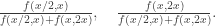
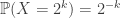
Let’s briefly consider an alternative example. It’s fairly easy to conjure up distributions which are almost surely finite but which have infinite expectation. For example for k=1,2,…, which is the content of the *St. Petersburg paradox*, another supposed paradox in probability, but one whose resolution is a bit more clear.

Anyway, let X and Y be independent copies of such a distribution. Now suppose your friend offers you an envelope containing amount X. You look at the value, and then you are offered the opportunity to switch to an envelope containing amount Y. Should you?

Well, if expectation is what you care about, then you definitely should. Because with probability one, you are staring at a finite value in your envelope, whereas the other unknown envelope promises infinite expectation, which is certainly larger than the value that you’re looking at.

Is this also a paradox? I definitely don’t think it is. The expectation of the content of your envelope is infinite, the expected gain is infinite with probability one, which is consistent with the expected content of the other envelope being infinite. [Note that you don’t want to be claiming that the expectation of X-Y is zero.]

An example density function

As an exercise that isn’t necessarily hugely interesting, let’s assume that f, the distribution of the smaller of the pair, is . So the mean of this smaller number is . Then, conditional on seeing x in my envelope, the expected value of the number in the other envelope is

(*)

Some straightforward manipulation shows that this quantity is at least x (implying it’s advantageous to switch) precisely when

That is, when . The shape of this interval should fit our intuition, namely that the optimal strategy should be to switch if the value in your envelope is small enough.

The point of doing this calculation is to emphasise that it ceases to be an interesting problem, and certainly ceases to be a paradox of any kind, once we specify f concretely. It doesn’t matter whether this is some true distribution (ie the friend is genuinely sampling the values somehow at random), or rather a perceived likelihood (that happens to be normalisable).

What if you should always switch?

The statement of the paradox only really has any bite if the suggestion is that we should always switch. Earlier, we discussed potential objections to considering the uniform prior in this setting, but what about other possible distributions f which might lead to this conclusion?

As at (*), we can conclude that when , we should switch on seeing x precisely if

Therefore, partitioning the support of f into a collection of geometric sequences with exponent 2, it is clear that the mean of f is infinite if everything is integer-valued. If f is real-valued, there are some complications, but so long as everything is measurable, the same conclusion will hold.

So the you-should-switch-given-x strategy can only hold for all values of x if f has infinite mean. This pretty much wraps up my feelings. If the mean isn’t infinite, the statement of the paradox no longer holds, and if it is infinite, then the paradox dissolves into a statement about trying to order various expectations, all of which are infinite.

Conclusions

Mathematical summary: it’s Bayes. Things may be exchangeable initially, but not once you condition on the value of one of them! Well, not unless you have a very specific prior.

Philosophical summary: everything in my argument depends on the premise that one can always describe the protagonist’s prior opinion on the contents of the pair of envelopes with a (possibly degenerate) distribution. I feel this is reasonable. As soon as you write down , you are doing a conditional expectation, and it’s got to be conditional with respect to something. Here it’s the uniform prior, or at least the uniform prior restricted to the set of values that are now possible given the revelation of your number.

Second mathematical summary: once you are working with the uniform prior, or any measure with infinite mean, there’s no reason why

with probability one (in terms of Y) should be surprising, since the LHS is (almost-surely) infinite while the RHS is almost surely finite, despite having infinite mean itself.

Birthday Coincidences and Poisson Approximations

This morning, Facebook was extremely keen to remind me via every available medium that four of my friends celebrate their birthday today. My first thought was that I hope they all enjoy their day, and my second thought was to ask what the chance of this was. I have about 200 Facebook friends, and so this struck me as an unlikely occurrence. But this problem has form, and it felt worthwhile to try some calculations to see if my intuition was well-founded.

Siméon Denis Poisson celebrated his 234th birthday on 21st June this year.

The classical birthday problem

The starting point is the question: how many friends do you have to have before you expect to start seeing anyone sharing a birthday? There are a ridiculous number of articles about this on the web already, so I will say little, except that I don’t want to call this the ‘birthday paradox’, because it’s not a paradox at all. At best it might be counter-intuitive, but then the moral should be to change our intuition for this type of problem.

Throughout, let’s discount February 29^th, as this doesn’t add much. So then, to guarantee having a shared pair of birthdays, you need to have 366 friends. But if you have a mere 23 friends, then the probability of having some pair that share a birthday is slightly greater than a half. The disparity between these two numbers leads to the counter-intuition. Some people might find it helpful to think that instead of counting friends, we should instead be counting pairs of friends, but I don’t personally find this especially helpful.

For me, thinking about the calculation in very slightly more generality is helpful. Here, and throughout, let’s instead take N to be the number of days in a year, and K the number of friends, or kids in the class if you prefer. Then, as usual, it is easier to calculate the probability that no two share a birthday (that is, that all the birthdays are distinct) than the probability that some two share a birthday. We could think of the number of ways to pick the set of birthdays, or we could look at the kids one-at-a-time, and demand that their birthday is not one of those we’ve already seen. Naturally, we get the same answer, that is

We’ve assumed here that all birthdates are equally likely. We’ll come back to this assumption right at the end. For now, let’s assume that both N and K are large, and we’ll try to decide roughly how large K has to be in relation to N for this answer to be away from 0 and 1. If we pair opposite terms up, we might approximate this by

In fact, AM-GM says that this is an overestimate, and a bit more care can be used to show that this is a good-approximation to first order. So we see that if for large N, we get a non-trivial limit.

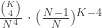
Challenges for four-way shared birthdays

So the original problem I posed is harder, because there isn’t (unless I’m missing something) a natural way to choose birthdays one-at-a-time, or describe the set of suitable birthday sets. There are two major obstacles in a calculation such as this. Firstly, the overlap of people, that is we might have five or more birthdays overlapping; secondly, the overlap of days, that is we might have several days with four (or more) birthdays. We’ll end up worrying more about the second situation.

We start by eliminating both problems, by asking for the probability that exactly four friends are born on January 1^st. The general form of this probability is . Now, if , this final term should not be significant. Removing this is not exactly the same as specifying the probability that at least four birthdays are on January 1^st. But in fact this removal turns a lower bound (because {exactly four}<{at least four}) into an upper (in fact a union) bound. So if the factor being removed is very close to one, we can use whichever expression is more convenient.

In the real life case of N=365, K=200, this term is not negligible. But accounting for this, we get that the probability of exactly four birthdays on 1^st January is ~0.0021. Our upper bound on the probability of at least four is ~0.0036.

But now that we know the probability for a given day, can we calculate to estimate the probability that we never have four-overlap? When we did our previous iterative calculation, we were using independence of the different kids’ birthdays. But the event that we have four-overlap on January 1^st is not quite independent of the event that we have four-overlap on January 2^nd. Why? Well if we know at least four people were born on January 1^st, there are fewer people left (potentially) to be born on January 2^nd. But maybe this dependence is mild enough that we can ignore it?

We can, however, use some moment estimates. The expected number of days with four-overlap is . So the probability that there is at least one day with four-overlap is at most ~0.77.

But we really want a lower bound. So, maybe we can borrow exactly the second-moment argument we tried (there for isolated vertices in the random graph) in the previous post? Here, the probability that both January 1^st and January 2^nd are four-overlapping is

From this, we can evaluate the expectation of the square of the number of days with four-overlap, and thus find that the variance is ~0.74. So we use Chebyshev, calling this number of days #D for now:

In our case, this unfortunately gives us an upper bound greater than 1 on this probability, and thus a lower bound of zero on the probability that there is at least one day with four-overlap. Which isn’t especially interesting…

Fairly recently, I spoke about the Lovasz Local Lemma, which can be used to find lower bounds on the probabilities of intersections of events, many of which are independent (in a particular precise sense). Perhaps this might be useful here? The natural choice of ‘bad event’ is that particular 4-sets of people share a birthday. There are such events, and each is independent of the collection of disjoint events. Thus we can consider using LLL if . Unfortunately, this difference of binomial coefficients is large in our example, and so in fact the LHS has order .

Random number of friends – coupling to a Poisson Process

All of these methods failed because without independence we had to use estimates which were really not tight at all. But we can re-introduce independence if we remove the constraints on the model. Suppose instead of demanding I have K friends, I instead demand that I have a random number of friends, with distribution Poisson(K). Now it is reasonable to assume that for each day, I have a Poisson(K/365) friends with that birthday, independently for each day.

If we end up having exactly K friends with this random choice, then the distribution of the number of 4-overlap days is exactly the same as in the original setup. However, crucially, if we end up having at most K friends with this random choice, the distribution of the number of 4-overlap days is stochastically dominated by the original distribution. So instead let’s assume we have Poisson(L) friends, where L<K, and see how well we can do. For definiteness, we’ll go back to N=365, K=200 now. Let’s say X is the distribution of birthdays in the original model, and for the distribution of birthdays in the model with a random number of friends

Then

(*)

Now we can write the crucial domination relation as

and then use an inequality version of the law of total probability to bound further as

This is a function of L, and in principle we could find its maximum, perhaps as . Here, though, let’s just take L=365/2 and see what happens. For (*) we get ~0.472.

To estimate , observe that this event corresponds to 1.4 standard deviations above the mean, so we can approximate using quantiles of the normal distribution, via the CLT. (Obviously this isn’t completely precise, but it could be made precise if we really wanted.) I looked up a table, and this probability is, conveniently for calculations, roughly 0.1. Thus we obtain a lower bound of . Allowing for the fairly weak estimates at various points, we still get a lower bound of around 0.4. Which is good, because it shows that my intuition wasn’t right, but that I was in the right ball-park for it being a ‘middle-probability event’.

Remarks and References

– The reason for doing the upper bound for the probability of exact 4-overlap is that the same argument for at-least-4-overlap would have given an upper bound of 1. However, this Poisson Process coupling is also a much better method for obtaining an upper bound on either event.

– Birthdays are not uniformly distributed through the year. The deviation is strong enough that even from the set of birth frequencies (rather than the sequence of birth frequencies), we can reject a null hypothesis of uniformity. Early September is pretty close to the maximum. Two comments: 1) this is the time of year where small variations in birth date have a big effect on education, especially in primary school; 2) we are 37 weeks into the year…

– It is known that 187 friends is the first time the probability of having at-least-4-overlap is greater than ½. You can find the full sequence on OEIS as A014088. I used to have about 650 Facebook friends, before I decided that I’d prefer instead the pleasant surprise of finding out what old acquaintances were up to when I next spoke to them. In this case, the median of the distribution of the largest number sharing a birthday would be seven.

– Eric Weisstein’s article on Mathworld is, in my opinion, the best resource for a mathematician on the first two pages of Google hits by at least two orders of magnitude. In the notation of this article, we were calculating . There are also some good general asymptotics, or at least recipes for asymptotics, in equations (17) and (18).

– The paper Methods for Studying Coincidences by Diaconis and Mosteller is, as one might expect, extremely readable, and summarises many results and applications, including several generalisations.

EGMO 2015

It’s been a while since I last wrote anything substantial. There have been some posts in the pipeline, but mainly I’ve been working hard on technical things that don’t translate very well into blog posts, and when I haven’t been working on those, have felt like doing non-maths.

Anyway, among other things which happened recently were the UK’s IMO selection camp in Cambridge during the last week of March, and the fourth European Girls’ Mathematical Olympiad in Belarus this past weekend. At the former, I was quite busy organising various things, and so gave a session based on some of my favourite problems about points and lines that I’ve used in the past. My hope was that with each problem in turn the students would actively invest time in thinking about whether the ideas each other were having seemed likely to be profitable. The aim was that being critical about your approach is a necessary skill once you start having lots of ideas for approaches.

This is hard to practise at school just by reading around, whether regarding competition material or generally. In the competition world, official solutions often contain unmotivated magic. This is reasonable, since they are supposed to be a minimal elementary demonstration of the problem’s validity. Motivation is a luxury which space and time sometimes doesn’t permit. And the solutions you find on, for example, Mathlinks often give the impression that the solvers know how to do 25,000 specific types of problem, and the sole task is to identify which type the latest one belongs to. Relating problems to ones you’ve seen before is important, but can hide, or at least dilute the actual ideas in some cases. Knowing that a specific inequality is a special case of a big machine allows you to claim a ‘solution’ but doesn’t help you identify the relevant ideas.

Later in the camp, a conversation arose concerning to what extent the younger staff found these elementary methods and problems easier now that they had experienced various levels of higher education in mathematics than when they were at school. It’s a complicated question, and I don’t think there’s a simple answer. I think the students might suspect that doing a university degree teaches you ‘advanced techniques’ which immediately simplify some of these problems. In rare examples this can be the case, but the majority of the time, I personally feel the only advantage I have is perhaps better instincts for whether something is or isn’t going to work.

Probably a good test would be Euclidean geometry. Adult olympiad staff typically come in two flavours: those who used to be good at geometry and feel out of practice; and those who weren’t good at geometry and certainly had no inclination to remedy this after they left school. I’m probably closer to the first category and I definitely feel out of practice, but also have minimal inclination to remedy this. Nonetheless, on the rare occasions I try these questions (and it’s not going to be for 4.5 hours at this stage…) my progress rate is probably comparable to when I was in sixth form. I’ve no idea how to turn this into a more concrete assessment, but there must be something about doing abstract maths all the time that prevents you forgetting how to do this, so presumably it should be at least as helpful in the types of problem with non-zero overlap with things I actually do. I won’t discuss geometry in the rest of this post, but I did also enjoy the geometry questions – it’s simply that I feel anything I have to say about them would be less useful than saying nothing.

In any case, I enjoyed trying the problems from Belarus in between bouts of typing, and thought I would write some brief comments about how I decided whether my ideas were good or not. To achieve this, I’ve looked at my rough, and will tell you the ideas which didn’t work, as well as some of the ones which did. I’ve paraphrased the statements slightly to avoid having too many LaTeX tags.

WARNING: what follows will spoil questions {2,4,5} if you haven’t already looked at them, but would like to.

Question 2 – A domino is a 2 × 1 or 1 × 2 tile. Determine in how many ways exactly n^2 dominoes can be placed without overlapping on a 2n × 2n chessboard so that every 2 × 2 square contains at least two uncovered unit squares which lie in the same row or column.

The wording of the question prompted me to consider splitting the board naturally into n^2 2 x 2 squares. I then thought about this ‘at least’ in the question, and concluded that for these 2 x 2 squares, it should be ‘exactly’.

I tried doing an unusual colouring, when I coloured half the black squares green, and half blue and tried to show that either only greens or only blues were covered, but this was clearly not true, or fixable. I then tried to do something similar for the other set of 2 x 2 squares (those whose vertices have (odd, odd) coordinates). Roughly speaking, if too few of the outer cells on the original board are covered, you can’t achieve the bounds on these odd inner squares. But this didn’t really give any useful information.

However, it did get me thinking about how what happens in the far top-left affects the rest of the board, and from there most of the ideas came quickly. I described a 2 x 2 square as N, E, S, W depending on which ‘half’ of the square was covered. Then if a square is N, all the squares directly above it must be also be N (*).

I then made two mistakes, and if we’re looking for reasons where experience is helpful, it was probably here, as I spotted them fairly quickly, rather than wasting ages and ages.

First, I decided that either all squares were {N,E} or all were {S,W} which seemed plausible when I had been focusing on the top-left. This gave an answer of , but after a bit more thought is clearly not symmetric enough.

Second, I thought condition (*) might be the only constraint, along with similar ones for E, S, W naturally too. I tried to count these using a similar method of enumerating lines between these regions, and I realised I didn’t know how to do these sensibly, for example if it looked like this:

This led to another bit of meta-maths that I probably wouldn’t have considered if I was 16. Namely, that the idea of counting these monotone lines across the 2n x 2n grid was too nice not to be useful. Also, if I couldn’t see a way to adapt it for this more complicated setup, my setup was probably wrong. This thought was useful, and then by thinking about the interface between {N,E} and {S,W}, then the other way round, it made sense that the configuration could be parameterised by two monotone lines between different pairs of corners, giving an answer of .

So, if it’s possible to give a reason why I could do this, it’s probably because I had an arsenal of ways to check an answer for plausibility, which saved wasting time on something wrong, and also because I trusted that the answer would be nice, which saved wasting time on something which was also wrong, and would probably have been very complicated to resolve.

Question 4 – Determine whether there exists an infinite sequence of positive integers satisfying .

So, my first reaction was ‘no way’. Why? Because everything’s determined by the first two terms, and I couldn’t think of any reason why a cool choice of the first two terms would force all of the sums to be perfect squares. It seemed just about possible that we could arbitrarily large finite sequences with this property. (Though this also turns out to be impossible.)

I imagine many contestants might have felt similarly and spent a while playing round with quadratic residues to get a sense for exactly how hard it is to make this work for the initial terms. But I was suspicious of the form of the recurrence. We know that if it had been defined linearly, then the terms would grow exponentially, but it’s natural to ask roughly how fast they grow in this example, even relaxing the restriction that the terms be integers.

The first observation was that they are indeed (strictly) growing! But how fast? Are there actually enough squares that every can be a different one? Note that the squares themselves satisfy a similar recurrence relation . So this seemed like a very good idea, and my instinct was that this should work, and I felt glad that I hadn’t pursued the quadratic residues approach.

From here we were basically home. I asked whether the sequence grows faster than the sequence , and the answer was no as

so if (after translating indices) , we have . This is clearly a problem or at best a very tight constraint if all the have to be perfect squares, so even though we aren’t completely finished, I am confident I can be in one or two lines, with a bit of care. Fiddling with small values of n looked like it would work, or showing that looking at a large enough initial subsequence that the effect of the first two terms dissipated, we must by the pigeonhole principle have , which is enough by a parity argument, using the original statement.

This final bit looks and feels a bit messy, but by this stage it really is just finding any argument to justify why a sequence which grows at most as fast as can’t actually be eventually.

Probably the reason I did this quickly was because I trusted my instinct for ‘no’, and also because there seemed a quick way to qualify *roughly* how this sequence grew. Sensibly approximating things, and deciding whether it’s appropriate to approximate them is definitely something I feel I’ve got better at during my PhD, so I guess this was helpful, then just try and throw back the important condition that the elements were integers at the very end.

Question 5 – Anastasia partitions the integers [1,2m] into pairs. Boris tries to choose one integer from each pair so that the sum is n. Given n and m, prove Anastasia can select pairs so that Boris can’t succeed.

So I wasted some thought time by imagining that n was fixed and trying to come up with ideas for the choice of pairs which might avoid n. It struck me that there was no reason why a a typical (uniformly chosen) pairing should avoid any particular n unless this value was particularly big or small.

How big or how small? Well Boris can always choose the bigger element of a pair, so the way to make the minimum maximum is to pair as (1,2), (3,4), … , (2m-1,2m). Conveniently, this also achieves the maximum minimum. These can be calculated as respectively. Suddenly this seems great, because we’ve actually solved the problem for a huge range of n, ie everything not within between these extrema.

The key step here was to start considering special pairings, chosen to give a reduced set of possible sums. Once we’ve had this idea, it makes sense to consider other different special pairings. The reason we got a small set of possible sums is that there’s lots of overlap. We can achieve lots of overlap by looking at the difference between elements in a pair, and making as many of these the same as possible. For, consider pairs (a,a+d), (b,b+d). Then it’s the same to take a and b+d as to take a+d and b, so we get the same sums in lots of different ways.

The other way to have as many differences the same as possible is to go for (1,m+1), (2,m+2), … , (m,2m). Conveniently, we can parameterise the sums now because at each choice, we decide whether to add an extra m or not, so the sum must be 1+2+…+m, plus some multiple of m. So we can defeat Boris, except when n is .

This is a good point to stop because what followed was basically book-keeping. We only have to consider a couple of specific cases when m is odd, and one when m is even, that happen not to fall into either of the categories we can now deal with. It wasn’t too hard to corrupt the examples we already have to deal with these.

The key here was responding to initial failure by trying to find any control at all over n. Perhaps given enough time I would have started trying special pairings? Equally, I might have tried small examples, which would not really have been hugely helpful for this question. In any case, trying to eliminate very small or very large n luckily worked well, as a) I didn’t need to use the word ‘very’ twice in the end; and b) the idea of looking at choices of pairings to minimise the number of sums quickly gave other useful deductions.

I also really enjoyed Question 3, though was suspicious that I’d used a bound a great deal weaker than one in the question. Along the way, I was trying something confusing and not especially useful that led me into some interesting theory about Latin squares, which I might write something about later in the week.

100k Views

When I started this blog, I implicitly made a promise to myself that I would be aiming for quality of posts rather than quantity of posts. Evaluating quality is hard, whereas one always feels some vague sense of purpose by seeing some measure of output increase. Nonetheless, I feel I have mostly kept this promise, and haven’t written that much solely for the sake of getting out another post. This post is something of an exception, since I noticed in the office on Friday that this blog was closing in on 100,000 page views. Some of these were not actually just me pressing F5 repeatedly. Obviously this is no more relevant an integer to be a threshold as any other, and one shouldn’t feel constrained by base 10, but it still feels like a good moment for a quick review.

Here are some interesting statistics over the years of this website’s existence.

• 175 posts, not including this one, or the three which are currently in draft status. This works out at about 4.7 posts a month. By some margin the most prolific period was May 2012, when I was revising for my Part III exams in Cambridge, and a series of posts about the fiddliest parts of stochastic calculus and network theory seemed a good way to consolidate this work. I’ve learned recently that PhDs are hard, and in fact it’s been a year since I last produced at least five posts in a month, if you discount the series of olympiad reports, which though enjoyable, don’t exactly require a huge amount of mathematical engagement.
• By at least one order of magnitude, the most viewed day was 17th August 2014, when several sources simultaneously linked to the third part of my report on IMO 2014 in Cape Town. An interesting point to note is that WordPress counts image views separately to page views, so the rare posts which have a gallery attached count well in a high risk / high return sense. In any case, the analytics consider that this day resulted in 2,366 views by 345 viewers. During a typical period, the number of views per visitor fluctuates between roughly 1.5 and 1.8, so clearly uploading as many photos of maths competitions as possible is the cheap route to lots of hits, at least by the WordPress metric.

• One might well expect the distributions involved in such a setup to follow a power-law. It’s not particularly clear from the above data about views per month since late 2012 whether this holds. One anomalously large data point (corresponding to the interest in IMO 2014) does not indicate a priori a power law tail… In addition, there is a general upward trend. Since a substantial proportion of traffic arrives from Google, one might naively assume that traffic rate might be proportion to amount of content, which naturally will grow in time, though it seems impractical to test this. One might also expect more recent posts to be more popular, though in practice this seems not to have been the case.
• The variance in popularity of the various posts has been surprisingly large. At some level, I guess I thought there would be more viewers who browse through lots of things, but such people would probably do so from the home page, so it doesn’t show up as viewing lots of different articles. There is some internal linking between some pages, but not enough to be a major effect.
• At either end of the spectrum, a post about coupling and the FKG inequality has received only 16 views in 2.5 years, while a guide to understanding the Levy-Khintchine formula has, in slightly less time, racked up 2,182 hits. There are direct reasons for this. Try googling Levy-Khintchine formula and see what comes up. In a sense, this is not enough, since you also need people to be googling the term in question, and picking topics that are hard but not super-hard at a masters level is probably maximising interest. But I don’t have a good underlying reason for why some posts should end up being more Google-friendly than others.
• In particular, quality of article seems at best loosely correlated with number of views. This is perhaps worrying, both for my reputation, and for the future of written media, but we will see. Indeed, two articles on the Dubins-Schwarz theorem and a short crib sheet for convergence of random variables, both get a regular readership, despite seeming to have been written (in as much as a blog post can be) on the back of an envelope. I also find it amusing that the Dubins-Schwarz theorem is always viewed at the same time of the year, roughly mid-February, as presumably it comes up in the second term of masters courses, just like it did in my own.
• By contrast, I remain quite pleased with the Levy-Khintchine article. It’s the sort of topic which is perfectly suited to this medium, since most books on Levy processes seem to assume implicit that their readers will already be familiar with this statement. So it seemed like a worthwhile enterprise to summarise this derivation, and it’s nice to see that others clearly feel the same, and indeed I still find some posts of this flavour useful as revision for myself.

• This seemed like a particularly good data set in which to go hunting for power-laws. I appreciate that taking a print-screen of an Excel chart will horrify many viewers, but never mind. The above plot shows the log of page view values for those mathematical articles with at least 200 hits. You can see the Levy-Khintchine as a mild anomaly at the far left. While I haven’t done any serious analysis, this looks fairly convincing.
• I haven’t engaged particularly seriously in interaction with other blogs and other websites. Perhaps I should have done? I enjoy reading such things, but networking in this fashion seems like a zero-sum game overall except for a few particularly engaged people, even if one gets a pleasing spike in views from a reciprocal tweet somewhere. As a result, the numbers of comments and out-going clicks here is essentially negligible.
• Views from the UK narrowly outnumber views from the US, but at present rates this will be reversed very soon. I imagine if I discounted the olympiad posts, which are sometimes linked from UK social media, this would have happened already.
• From purely book-keeping curiosity, WordPress currently thinks the following countries (and territories – I’m not sure how the division occurs…) have recorded exactly one view: Aaland Islands, Afghanistan, Belize, Cuba, Djibouti, El Salvador, Fiji, Guatemala, Guernsey, Laos, Martinique, Mozambique, New Caledonia, Tajikistan, US Virgin Islands, and Zambia. Visiting all of those would be a fun post-viva trip…

Conclusion

As I said, we all know that 100,000 is just a number, but taking half an hour to write this has been a good chance to reflect on what I’ve written here in the past three years. People often ask whether I would recommend that they start something similar. My answer is ‘probably yes’, so long as the writer is getting something out of most posts they produce in real time. When writing about anything hard and technical, you have to accept that until you become very famous, interest in what you produce is always going to be quite low, so the satisfaction has to be gained from the process of understanding and digesting the mathematics itself. None of us will be selling the musical rights any time soon.

I have two pieces of advice to anyone in such a position. 1) Wait until you’ve written five posts before publishing any of them. This is a good test of whether you actually want to do it, and you’ll feel much more plausible linking to a website with more than two articles on it. 2) Don’t set monthly post count targets. Tempting though it is to try this to prevent your blog dying, it doesn’t achieve anything in the long term. If you have lots to say, say lots; if you don’t, occasionally saying something worthwhile feels a lot better when you look back on it than producing your target number of articles which later feel underwhelming.

I don’t know whether this will make it to years, but for now, I’m still enjoying the journey through mathematics.

A Month in Vancouver

I’ve spent the past ~3 weeks at the University of British Columbia in Vancouver, working on some projects related to forest fires and frozen percolation with Balazs Rath. In advance, I’d imagined that this might be a prolific time for new articles on this blog, but in the end it was more like the exact opposite. After spending all of every day playing with technical details on our models (which do not lend themselves naturally to informal writing…) if I felt like doing maths in the evenings, it was more important to keep working on the questions in hand.

Anyway, I had a great time mathematically and otherwise, so I feel a shameless tourism post is justified to report what I enjoyed most about Vancouver.

Asian Food

It sounds ridiculous to return from a trip and reference this as the highlight, but the most noticeable long-term result of a month in Vancouver is that I will probably never be able to order sushi in the UK again. The typical house roll cost about £3 and contained so much seafood that it was essentially impossible to manipulate. Or maybe that was just my (lack of) chopstick skills? Anyway, as I’ve observed in other parts of Canada, groceries bizarrely expensive relative to eating out, at least relative to Europe. By my third week I had basically given up and found a different East Asian cuisine every other night. I ate Japanese, Chinese, Korean, Thai, Malaysian, Taiwanese, Vietnamese and others that didn’t feel constrained by a single national identity. All were uniformly excellent, unfailingly welcoming, and made commendable efforts to include smoked salmon in every single dish.

Outdoor Pursuits

For a country where a donut shop is an integral part of the national identity, the total absence of fat people was immediately noticeable. In their place was a city where everyone seemed to go running, hiking, skiing, quad-biking, skidoo-ing and so on at the slightest opportunity. I haven’t seen that much lycra since breakfast in college on the morning of May Bumps…

For a major world city, the wilderness was tantalisingly close, and remarkably accessible. The public transit system spread far into the mountains and up the coast, and offered you any 90 minutes worth of travel for $2. A breezy ferry trip across the sound to Bowen Island offered the chance to hike up Mt Gardner, an unrelenting and totally solitary trek up through the pine forest. I was conscious that if I slipped somewhere, there wouldn’t be much left to find once the bears had got to me, but the views over the inlet from the summit made it all worthwhile. A trip to Mt Seymour on Victoria Day, then down past the vertigo-inducing Lynn Suspension bridge and a trail back towards civilisation was equally successful. On both occasions, felt I’d very much earned that donut.

UBC

Of course, the main reason for the trip was to do worthwhile mathematics, and I certainly haven’t experienced a nicer university campus to do exactly that. A five minute walk and 500 steps away from the Wysteria-covered maths department is the 7km long Wreck Beach, a sunny haven for Vancouver’s hipsters and nudists, protected from direct exposure to the Pacific by Vancouver Island. Of more interest to me were the 30km or so of trails through the forest in the Pacific Spirit Regional Park, directly across the road from where I was staying in Wesbrook Village at the south end of the campus.

Most importantly, I’m extremely grateful for the invitation to work at UBC for these past few weeks. It’s been productive, and an excellent opportunity to meet some new people and learn about some interesting aspects of probability. I very much hope an opportunity will arise to go back soon!

Guess 2/3 of the average

The following problem was doing the rounds on some email lists in Oxford this week:

“You and a group of colleagues are all invited to pick an integer between 0 and 100. The average x is calculated, and the person whose guess is unique and comes closest to 2x/3 (among the unique guesses) is declared the winner.”

Although it wasn’t specified in the setting, one assumes that if two unique guesses were equally close to 2/3 of the average, then the two participants shared the prize.

In any case, it is interesting to ask the question, what is the optimal strategy?

I don’t know very much about game theory, so I’m going to say some things that I hope are true. I don’t claim that this is the best or even a good way of thinking about the situation. If we break the problem down into two parts, we have two of the more famous problems in game theory. To consider the first part, we remove the requirement that the winner’s guess be unique, and allow the participants to pick any real number between 0 and 100.

It seems to me there are three ways to do this. Let’s say we have K possible winners who guessed closed to 2x/3. We could give each of them the fixed prize, say £1. Or we could give each of them £1/K, or we could choose one at random and give them £1. I claim that the latter two methods are essentially the same, and so will ignore the third possibility.

Note that 2x/3 will definitely be at most 200/3. Suppose I pick a real value y that is greater than 200/3. What would happen if instead I picked 200/3? Well the value of x would decrease slightly. How much it decreases would depend on the number of people playing the game. It is not hard to check that we end up closer to 2x/3 if we pick 200/3 instead of y. Let’s call .

We might say that the strategy “pick ” dominates the strategy “pick y”, because we always do at least as well with the first strategy as the second, regardless of what the other players do, and indeed in some cases do strictly better. Now comes the potentially philosophical bit. We have concluded that it would be irrational for us to pick any number greater than . We also know that the email was sent to mathematicians in Oxford, whom we might hope we could safely assume were equally rational. So now we are playing the same game as before, only with the bounds that we should pick a number between 0 and . We can then apply exactly the same argument to show that it would be irrational to pick any number greater than . This equally applies to all the other agents, and so we continue, showing that for any k, it is irrational to pick any number greater than . In conclusion, the only rational strategy is to pick 0, and hence everyone will do this.

For the prize structure suggested, this is a Nash equilibrium, since no-one can improve their winnings by changing strategy (with everyone else’s kept the same). This principle is in general referred to as iterated elimination of dominated strategies. The assumption that, not only are players rational, but that all players know that all other players are rational, and all players know that all players know the others rational and so on, is called Common Knowledge of Rationality. This doesn’t seem hugely controversial in this artificial setting, but it is not hard to think of examples where this might not hold. For example, some players might be facing the same situation, but have different utility functions, so especially if there is some randomness in the dynamics, people will have different ‘rational’ opinions concerning strategies, and unless you know their utility functions, it might seem like the other players are not acting rationally.

This argument works equally well with integers. We first eliminate all possibilities greater than 67, and then keep dividing by 2/3, but we have to take the ceiling function to get the new upper bound. As a result, after repeated application of this idea, we conclude that the only rational strategies are to pick 0 or 1.

It can be seen that neither strategy dominates the other. If more than ¾ of the agents choose 1, then choosing 1 is the optimal strategy; if less than ¾ choose 1, then choosing 0 is better. If exactly ¾ choose 1 then everyone wins. There are, however, only two Nash equilibrium, given by everyone choosing 1, and everyone choosing 0. It is tempting to argue that we might expect roughly ½ the agents to choose 1, and so our better option is to choose 0. But we are assuming the other agents are rational, and there is no a priori reason why picking 0 or 1 with probability ½ each should be the rational thing to do.

However, choosing randomly is a possible strategy. In this setting, it becomes harder to talk about Nash equilibria. When there are just two agents, the set of even random strategies for each agent is relatively manageable, but when there is some arbitrary number of players, the set of possible strategies might be very complicated indeed.

The final stage of this integer problem is morally equivalent to playing a game where everyone has to pick 0 or 1, and you win if you are in the majority. For this problem, it is clear that the only Nash equilibria are for everyone to pick either 0 or 1. If the winners share the prize-money equally, then this game has the interesting property that every configuration is Pareto optimal. This means that no-one can improve their winnings without causing someone else’s situation to decrease. When it comes to deciding what to do, with no knowledge of other people’s strategies, we have made little progress. At least here the symmetry between 0 and 1 makes it clear how little progress we can make. The only thing we can say is that if the utility is concave (a generally reasonable assumption), then by conditioning on what everyone else does, an optimal strategy is to pick 0 with probability 1/2.

The problem with saying anything sensible in these sorts of problem with a zero-sum condition (as we effectively have if the winnings are shared) is the symmetry between all the players. Given any strategy, if everyone used that strategy, then everyone would win 1/N in expectation. This applies equally well if we add the condition that the winner has to pick something unique.

The only question we can perhaps say something about occurs if we say that no-one wins the original game if there are no unique integer answers. Then it is worth considering which strategy could everyone adopt so as to minimise the probability of this happening. For the reasons given above, we should indeed force everyone to take the same strategy, which we can interpret as a distribution on the integers. So which distribution on the integers between 1 and k maximises the probability of having at least one unique value?

We also need to know how many people are playing, so let’s say this is N. I don’t know how to solve the general problem, but I can say something if we fix either k or N and then let the other one go to infinity.

If we fix the number of people and let k go to infinity, then we can get arbitrarily close to probability one by using the uniform distribution. Indeed, any sequence of distributions where the probabilities converge uniformly to zero ( ie ) has this property.

The case where k is fixed and the number of players goes to infinity is a bit trickier. Essentially, if we choose any fixed distribution, the event we seek becomes less and less likely as the number of agents grows. It is equivalent to demanding that if we roll a dice a million times, we only see precisely one six. If we replace a million by larger numbers, this probability decays exponentially.

If we want to maximise the probability of getting precise one agent choosing value 1, we observe that the number of agents choosing that value is binomial(N,p), where p is the probability of that value. If p=o(1/N) then asymptotically, with high probability the number of 1s is 0. If p=w(1/N) then asymptotically, with high probability, the number of 1s is . Taking , the asymptotic distribution of the number of 1s is Poisson with parameter . We can solve to see which value of maximises the probability of getting a single 1. It turns out, unsurprisingly after considering the expectation of the corresponding pre-limit binomial distribution, that this maximum is achieved at .

So note now that if we take the probabilities of picking 1 and 2 both to be 1/N, we get two Poisson random variables asymptotically. For a similar argument to the construction of the Poisson process from independent infinitesimal increments, the covariance of these tends to 0. So I conjecture, and I reckon it is probably not too hard to come up with a formal proof that for large N, the optimal distribution looks like:

or some permutation of that.

Related articles

• Gauss’s lemma (polynomials) (cozilikethinking.wordpress.com)
• An interesting inequality (sirjackshen.wordpress.com)
• Group (kantandcantor.wordpress.com)
• The Smartest Gambler (maxktricks.wordpress.com)

The Top-to-Random Shuffle

This article is based on a talk I gave to the Maths Society at St Paul’s School on Monday. It may turn into a short series if I have time before I go to ALEA in Luminy near Marseille on Saturday.

My original plan had been to talk about riffle-shuffling, and some of the interesting mixing time themed results one can obtain. As a motivating example, I began by discussing the simpler top-to-random shuffle, and this proved sufficiently interesting to occupy the time I had been allowed (and mea culpa a bit more). It therefore seems worth writing a hopefully moderately accessible blog post on the subject. The aim of this post at least is to discuss the idea that repeatedly shuffling brings a pack of cards close to randomness. We have to settle on a definition of ‘close to randomness’, and find some ways to calculate this.

Suppose we are playing some bizarre card game where it is necessary that three cards labelled, uncontroversially, 1, 2 and 3 need to be placed in a random order. If we are organised, we can write down all the ways to do this in a list:

123, 132, 213, 231, 312, 321.

We want to select each of these with equal probability. We could for example use a dice. Most relevantly, even a computer as ancient as my laptop is very happy simulating a random choice from this set. (Now is not the time to talk about exactly how pseudo-random or otherwise this choice would be.)

Of course, when we play a sensible card game we have not three cards, but fifty-two. So the approach described above still works in theory, but no longer in practice, as the list of possible arrangements now has size 52!. Recall this is defined to be

The reason we get this particular expression is that when we are choosing the first card, we have 52 possible choices. Then, regardless of what this first card actually is, there are precisely 51 cards left from which to choose the second card. So there are 52×51 ways to pick the first two cards in the arrangement, and so on, giving the answer. We can approximate how large 52! is by counting powers of ten rather crudely. It seems reasonable that it should be about . Note that the number of atoms in the universe is *only* about , so if we are going to write down this list, we better have very compact handwriting! But being serious, this number is way too large to realistically compute with, so we have to come up with some cleverer methods.

One way is to spread the cards out on a table then pick them up one at a time, ensuring at all times that the choice of card is uniform among those currently present, and not related to any of the past choices. This is relatively easy for a computer, but hard for a human, and certainly deeply tedious for anyone waiting to receive their hand!

So we seek a different approach, namely an algorithm for shuffling. Our aim is to introduce overall randomness by repeatedly applying some simple but random process. Note we have to be careful about our definition of ‘random’ here. The permutation 123456 is just as ‘random’ as the permutation 361524. That is, if they are fixed, then they are not random at all. Just because it is easier to decribe one of them verbally does not mean it is less random. For example, if I am trying to cheat at poker, then I might be able to if I knew the exact order of the cards in the pack before the dealer dealt. It wouldn’t matter what that order was. I would have to adjust my strategy based on the order, but it wouldn’t affect the fact that I had a massive advantage!

The shuffling algorithm to be discussed here is the top-to-random shuffle. Like all the best things in life, this does exactly what it says on the tin. At a given time, we remove the top card from the deck at present, and insert it at a randomly chosen point in the deck. This could be on the bottom, and it could also be back on the top. It feels like this possibility to remain constant can’t possibly help us, but later we will discuss why we need this.

In any case, it feels natural that if we keep applying this procedure, the arrangement of the deck should start to get more and more random, in the sense that knowing the original arrangement will tell us successively little about the current arrangement as time progresses. But we need to find a way to quantify this if we are to do any mathematics.

When we are talking about real numbers, it is fairly clear what it means if I say that the numbers 2, 1.1, 1.01, 1.001 and so on are getting closer and closer to 1. Indeed we can measure the distance along the number line between each term and 1, using the absolute difference. It is not so clear how to compute the distance between two probability distributions. Bearing in mind the fact that a distribution on the set of permutations of cards is defined to be a set of 52! probabilities that sum to 1, there will be a 52!-1 dimensional space (eg the plane is two-dimensional, the world is three-dimensional, *and so on* – whatever that means) where we have a nice distance formula already.

But this is not what we will choose to use. Rather we return to the cheating-at-poker analogy. Suppose I am playing some sort of game involving the pack of cards with my enemy. He or she thinks the deck is perfectly random, but I know the actual distribution. How big a profit can I make by exploiting this knowledge? This will be our measure of how far a distribution is from uniform. It turns out that this will coincide precisely with the formal definition of total variation distance, but that language belongs to a different level of rigour and is not relevant here.

What is relevant is an explanatory example. Suppose we start with the arrangement 12345678. We are now going to perform one iteration of the top-to-random shuffle. The outcome might, for example, be 23456178, if we insert the 1 between the 6 and the 7. Note there were 8 places for the card to go, so the probability of this particular outcome is 1/8. Now let’s see how I might use my knowledge of the distribution to my advantage. Suppose I suggest the bet that the bottom card is an 8. My enemy thinks the stack is uniformly randomly arranged, so the probability of this is 1/8. On the other hand, I know that the only way the 8 might disappear from the bottom is if I place the 1 under it, which happens with probability 1/8. So in fact, I know the probability of this event is 7/8, which gives me an advantage of 3/4. In fact, I could come up with bets that do even better than this, but they are less simple to describe verbally.

At what point do I lose this advantage? Well, we said that the probability that the 8 leaves the bottom of the stack is 1/8. And it will continue to be 1/8 on every turn where it is at the bottom. Recalling that the outcomes of successive shuffles are independent, note this is reminiscent of rolling a dice until a six comes up. The number of rolls required to get the six is an example of a geometric random variable. I don’t want to spoil S1 (or whichever module) by going into too much detail, but it turns out that if the probability of an event happening on a single go is p, then the average time we have to wait is 1/p. So 1/(1/8)=8 of course, and this is how long we typically have to wait before the bet I placed before becomes much less effective.

Now seems like a good time to stop talking about 8 cards and start talking about n cards. Obviously, in practice, we will want n to be 52. Anyway, by the same argument as before, it takes on average n iterations before the bottom card leaves the bottom. This is important, because after then, my bet that the bottom card is n is no longer so effective. However, I could equally place a bet that one of the bottom *two* cards is n.

So we consider how long it takes before n is no longer one of the bottom two cards. Well certainly we need to wait until it is no long *the* bottom card, which takes time n on average. Then, once it is second bottom, there is now a 2/n chance that we move the previously top card below it, so by the same argument as before, the time for this to happen is n/2 on average. If we want this effect to disappear, we have to wait until the original bottom card is in fact at the top of the pile for the first time, and by extending our previous argument, the average time for this is

Fortunately, we have tools for approximating this sort of sum, in particular integration, which is the practice of finding the area under certain curves. It turns out that the answer is roughly n log n. You can think of as log n a measure of the number of digits required to write out n. (This is not the exact definition but it will do for now. In any case, log n gets larger as n gets larger, but not very fast.) There’s a lot more about this in my previous post on the coupon collector problem, from a more technical point of view.

The next question will be to prove that it is actually quite well shuffled by this time, but that’s for another post. The other question to ask is whether this is satisfactory overall? For n=52, the number of operations we have to perform is about 230, which is fine for a computer, but deeply tedious for anyone sitting at a casino table waiting for the next hand. So next time we’ll talk about the riffle shuffle, which seems to introduce a lot of randomness in each go, but we’ll also see that we have to be careful, because the randomness may not be as great as our intuition suggests.

Related articles

• Your Old Deck of Cards is Unique (alwaysephemera.com)
• Hyena’s Top Titillating Spoiler Cards (hextcgshuffle.com)
• For My Poker Friends: Shuffling 52 Cards (norberthaupt.com)
• A Pretty Trick (the1642goodwyfe.wordpress.com)

Responding to the Monty Hall Problem

It’s been a while since I got round to writing anything, so I’m easing myself back in by avoiding anything too mathematically strenuous. Shortly after my last post, there was a nice clip on Horizon featuring Marcus du Sautoy explaining the famous Monty Hall Problem to the ever-incredulous Alan Davies. The BBC article here shows the clip, and then an excellent account by probabilist John Moriarty explaining the supposed paradox.

Recall the situation. A game show is hosted by Monty Hall. At some point, to decide the grand prize, or whatever, a contestant plays the following lottery. There are three doors, and three prizes, one behind each. One of the prizes is worthwhile, normally a car, while the other two are rubbish. For reasons I don’t understand, it is normally said that behind the other two doors are goats. Anyway, MH knows where the car is from the beginning. Then the contestant picks a door, but doesn’t open it yet. MH then dramatically opens a different door, revealing a goat. The contestant then has the option to stick with his original choice, or switch to the third door. What should he or she do?

So the natural error to make is that since one possibility has been eliminated, since the remaining two were a priori equally likely, they should still be equally likely, and hence each occur with probability 1/2. So it makes no difference whether you stay or switch. But, of course, as well as removing information (ruling out one door), we have also gained information. The fact that MH chose to reveal that door, rather than the potential third door is important.

In my opinion, the best way to think about this is to imagine you are the host. The nice thing about being in this position is that then you can imagine you know everything about the configuration in advance, so are less likely to fall foul of counter-intuitive conditional probabilities. Anyway, there’s loads of symmetry, so from my point of view as the host, I only care whether the contestant initially selects the right door or the wrong door. If he selects the wrong door, then I need to open the ONLY OTHER wrong door. In other words, I have no choice in what I do next. I open the other wrong door. Therefore in this case the contestant should switch. If the contestant in fact selects the right door initially, I then have a choice about which door to open. However, it doesn’t really matter which I pick, by symmetry, and in either case the contestant would do better to stay with his original choice. Note that we have defined the outcome entirely by the initial choice. And as the host, I knew where the car was at the start, so from my point of view, unless he had somehow cheated, the contestant always had a 1/3 chance of guessing correctly. So it is better to switch 2/3 of the time.

The BBC’s weekly collation feature, The Loop, printed a couple of responses to the article. This is one:

“I believe that the problem is a game of two halves. In the first instance you have a 1:3 chance of getting the prize. Once you’ve made your initial choice, even though the ‘box’ contents remain the same, one ‘false’ choice is removed and you are then offered the chance to choose again. There is a play on words here, perhaps, with the option to ‘switch’. Effectively you are being asked to make a choice of 1:2. Now, if this is always going to happen then the odds of you winning the prize in the first instance is 1:2, as it doesn’t really matter whether or not you choose correctly the first time – one ‘false’ is going to be removed and you’ll be presented with just two options. It’s mind trickery. The first choice is totally irrelevant because you will always end up having to pick one option from two in order to attain the prize. In my humble opinion.”

I highlight this not to inspire contempt, since it is an easy mistake to make, even after reading as nice an explanation as Moriarty’s. Rather it is an excellent example of how using too many words can convince you an argument is complete before you’ve really made any concrete statement at all. Note that the sentences beginning ‘Effectively…’, ‘Now, if this…’ and ‘The first choice…’ all say exactly the same thing, which is, to use inappropriately formal terminology, exactly what the writer is trying to prove. The padding of ‘mind trickery’ and ‘humble opinions’ is as close as a maths argument can ever really come to an ad hominem.

So I was trying to come to a clean conclusion about exactly why the Monty Hall problem does such a good job at generating confusion. I think the following aspects of the set-up are important:

1) In general, people often get confused about the meaning of ‘random’. In some sense, the sequence 416235 is more random than the sequence 123456. However, typically, we use ‘random’ to mean ‘not determined in advance’. The key is that the bit where MH reveals a goat is not a random action. Whatever you do initially, you know that this will happen. So the fact that it does actually happen should not add extra information.

2) This fact is compounded by the time-steps at which decisions have to be made. It feels like the arc of the narrative is directing everything towards this final choice, which feels very separate from the initial choice. You can imagine the dramatic music that undoubtedly plays as MH opens the appropriate door, and the camera pans back to the contestant making their decision. All of which is an excellent way to suggest that something complicated has happened, when in fact in terms of what we are interested in overall, nothing has happened.

A point I hadn’t thought about before was that it is important that MH knows what happens in advance. Let’s develop this point and consider what happens if MH in fact has no knowledge of where the car is, and chooses a door at random. We will still assume that he must choose a different door to the one that the contestant originally chose.

Then, 1/3 of the time the contestant picks a goat, and MH picks the car, so he gets a goat whether he stays or switches. 1/3 of the time, the contestant picks a goat, and MH picks the other goat, so he should switch. And 1/3 of the time, the contestant originally picks the car, and then by default MH picks a goat, so he should stay. So, overall, it is equally preferable to stay as to switch.

I guess the morals of this story are: “be careful with conditional probabilities; sometimes apparently new information doesn’t change anything; and that it’s probably not a good idea to get into a discussion about the Monty Hall problem with a skeptic unless you have a piece of paper to hand on which to draw a probability table.”

Related articles

• Lesson 4: The Monty Hall Problem (heiyinsin.wordpress.com)
• The Monty Hall Problem- Counter-intuition (13laic1.wordpress.com)
• The Monty Hall Problem (robinsoons.wordpress.com)
• Goat or No Goat: applying the Monty Hall problem to Deal or No Deal (theunforgivingminuteuk.wordpress.com)
• Monty Hall problem: The probability puzzle that makes your head melt (misbehavedwoman.wordpress.com)
• The probability puzzle that makes your head melt (bbc.co.uk)
• How Randomness Rules Our World (kennethmutuma.wordpress.com)
• The Loop: Monty who? (bbc.co.uk)

PS. A final moral is that, based on the links WordPress suggested, at least 10% of the internet is devoted to explanations of the Monty Hall problem…