Nested Closed Intervals

Th UK team for this year’s International Mathematical Olympiad in Santa Marta, Colombia, has just been selected. For details, see the BMOC website.

During the selection camp, which was hosted at Oundle School near Peterborough, we spent a while discussing analytic questions that typically lie outside the scope of the olympiad syllabus. Furthermore, incorrect consideration of, for example, the exact conditions for a stationary point to be a global maximum, are likely to incur very heavy penalties if a candidate has attempted a solution using, for example, Lagrange multipliers. As a result we have a dilemma about how much analysis to teach during the training process: we want the students to be able to use sophisticated methods if necessary; but we don’t want to spoil the experience of learning this theory in a serious step-by-step manner as first year undergraduates.

This post does not present a solution to this dilemma. Rather, I want to discuss one question that arose on the last day of exams. Because the statement of the question is currently classified, I will have to be oblique in discussion of the solution, but this shouldn’t distract from the maths I actually want to talk about.

The setup is as follows. We have a sequence of nested closed intervals in the reals, that is:

We want to demonstrate that there is some real number that lies in all of the intervals, that is . This feels intuitively obvious, but some form of proof is required.

First, what does closed mean? Well a closed interval is a closed set, but what about, for example, ? It turns out that it is most convenient to define an open set, and then take a closed set to be the complement of an open set.

The best way of thinking about an open set is to say that it does not contain its boundary. This is certainly the case for an open interval or an open ball. It is not immediately clear how to extend this to a general definition. But note that if no point in the set X can be on the boundary, then in all the natural examples to consider there must some finite distance between any point and the boundary. So in particular there is a small open ball centred on x that is entirely contained within X. This is then the definition of an open set in a metric space (in particular for some ).

Note that it is not a sensible definition to say that a closed set has the property that there is a closed ball containing each point. Any open set has this property also! For if there is an open ball of radius R around a point x, then there is a closed ball of radius R/2 around that same point. So we really do have to say that a set is closed if the complement is open. Note that in , a closed interval is closed, and a finite union of closed intervals is closed, though not a countable union as:

Now we know what a closed set is, we can start thinking about the question.

First we remark that it is not true if we allow the interval to be unbounded. Obviously . Note that even though it appears that these sets have an open upper boundary, they are closed because the complement is open. This will not be a problem in our question because everything is contained within the first interval and so is bounded.

Secondly we remark that the result is not true if we move to a general host set. For example, it makes sense to consider open and closed sets in the rationals. For example, the open ball radius 1 either side of 1/2 is just all the rationals strictly between -1/2 and 3/2. We could write this as . But then note that

cannot contain any rational elements, so must be empty.

There was various talk that this result might in general be a consequence of the Baire Category Theorem. I think this is overkill. Firstly, there is a straightforward proof for the reals which I will give at the end. Secondly, if anything it is a lemma required for the proof of BCT. This result is often called Cantor’s Lemma.

Lemma (Cantor): Let X be a complete metric space, and let be a nested sequence of non-empty closed subsets of X with . There there exists such that

Translation: for ‘complete metric space’ think ‘the reals’ or . The diameter is, unsurprisingly, the largest distance between two points in the set. For reasons that I won’t go into, the argument for the olympiad question gave so this certainly holds here.

Proof: With reference to AC if necessary, pick an element for all n. Note that by nesting, . As a result, for m>n the distance . This tends to 0 as n grows. The definition of complete is that such a sequence then has a limit point x.

Informally, completeness says that if a sequence of points get increasingly close, they must tend towards a point in the set. This is why it doesn’t work for the rationals. You can have a sequence of rationals that get very close together, but approach a point not in the set, eg an irrational. We use the definition of closed sets in terms of sequences: if the sequence is within a closed set, then the limit is too. This could only go wrong if we ‘leaked onto the boundary’ in the limit, but for a closed set, the boundary is in the set. This shows that for each n, and so $x\in\cap_n F_n$. But if there is another point in , then the distance between them is strictly positive, contradicting the claim that diameter tends to 0. This ends the proof.

Olympiad-friendly version: I think the following works fine as a fairly topology definition-free proof. Consider the sequence of left-boundaries

This sequence is non-decreasing and bounded, so it has a well-defined limit. Why? Consider the supremum. We can’t exceed the sup, but we must eventually get arbitrarily close, by definition of supremum and because the sequence is non-decreasing. Call this limit a. Then do the same for the upper boundaries to get limit b.

If a>b, then there must be some , which is absurd. So we must have some non-empty interval as the intersection. Consideration of the diameter again gives that this must be a single point.

Related articles

• Confidence interval for a single proportion (statsmethods.wordpress.com)
• An interesting inequality (sirjackshen.wordpress.com)
• Littlewood’s Three Principles (shinyetemon.wordpress.com)
• I just can’t resist: there are infinitely many pairs of primes at most 59470640 apart (sbseminar.wordpress.com)
• Almost all continuous functions are nowhere differentiable (chiasme.wordpress.com)

Local Limits

In several previous posts, I have talked about scaling limits of various random graphs. Typically in this situation we are interested in convergence of large-scale properties of the graph as the size grows to some limit. These properties will normally be metric in flavour: diameter, component size and so on. To describe convergence of these properties, we divide by the relevant scale, which will often be some simple function of n. If we are looking to find an actual limit object, this is even more important. This is rather similar to describing properties of centred random walks. There, if we run the walk for time n, we have to rescale by to see the fluctuations on a finite positive scale.

One of the best examples is Aldous’ Continuum Random Tree which we can view as the limit of a Galton-Watson tree conditioned to have total size n, as n tends to infinity. Because of the exploration process or contour process interpretation, where these functions behave rather like a random walk, the correct scaling in this context is again . The point about this convergence is that it is realised entirely as a convergence of some function that represents the tree. For each finite n, it is clear that the tree with n vertices is a graph, but this is neither clear nor true for the limit object. Although it does indeed have no cycles, if nothing else, if the CRT were a graph it would have [0,1] as vertex set and then would be highly non-obvious how to define the edges.

Local limits aim to give convergence towards a (discrete) infinite graph. The sort of properties we are looking for are now local properties such as degrees and correlations of degrees. These don’t require knowledge of the whole graph, only of some finite subset. First consider the possibility that the sequence of deterministic graphs has the property:

where denotes an induced subgraph. Then it is relatively clear what the limit should be, as it is well-defined to take a union. This won’t work directly for a limit of random graphs, because the above relation in probability doesn’t even really make sense if we have a different probability space for each finite graph. This is a general clue that we should be looking to use convergence in distribution rather than anything stronger.

In the previous example, suppose the first finite graph consists of a single vertex v. If the limit graph (remember this is just the union, since that is well-defined) has bounded degrees, then there is some N such that contains all the information we might want about the limiting neighbourhood of vertex v. For some larger N, contains all the vertex and edges within distance r from our starting vertex v that appear in the limit graph.

This is all the motivation we require for a genuine definition. We will define our limit in terms of neighbourhoods, so we need some mechanism to choose the central vertex of such a neighbourhood. The answer is to consider rooted graphs, that it a graph with an identified vertex. We can introduce randomness by specifying a random graph, or by giving a distribution for the choice of root. If G is finite, the canonical choice is to choose the root uniformly from the set of vertices. This isn’t an option for an infinite graph, so we define the system as (G, p) where G is a (for now deterministic) graph, and p is a probability measure on V(G).

We say that the limit of finite is the random rooted infinite graph (G, p) if the neighbourhoods of around a randomly chosen vertex converge in distribution to the neighbourhoods of G around p. Formally, say if for all r>0, for any finite rooted graph (H,w), the probability that (H,w) is isomorphic to the ball of radius r in centred at randomly chosen $v_n$ converges to the probability that (H,w) is isomorphic to the ball of radius r around v in (G,v), where v is distributed according to measure p.

Informally, we might say that if we zoom in on an average vertex in for large n, the neighbourhood looks the same as the neighbourhood around the root in (G, p). We now consider three examples.

1) When we talk about approximating the component size in a sparse Erdos-Renyi random graph by a branching process, this is exactly the limit sense we mean. The approximation fails if we fix n and take the neighbourhood size very large (eg radius n), but for finite neighbourhoods, or any radius growing more slowly than n, the approximation is good.

2) To emphasise why rooting the finite graphs makes a difference, consider the full binary tree with n levels (so vertices). If we fix the root, then the limit is the infinite-level binary tree, though this isn’t especially surprising or interesting.

Things get a bit more complicated if we root randomly. Remember that the motivation for random rooting is that we want to know the local structure around a vertex chosen at random in many applications. If we definitely know what vertex we are going to choose, we know the local structure a priori. Note that in an n-level binary tree, vertices are leaves, not counting the base of the tree, and are distance 1 from a leaf, and are distance 2 from a leaf and so on.

This gives us a precise description of the limiting local neighbourhood structure. The resulting limiting object is called the canopy tree. One picture of this can be found on page 6 of this paper. A verbal description is also possible. Consider the set of non-negative integers, arranged in the usual manner on the real line, with edges between adjacent elements. The distribution of the root will be supported on this set of vertices, corresponding to the distance from the leaves in the pre-limit graph. So we have mass 1/2 at 0, 1/4 at 1, 1/8 at 2 and so on. We then connect each vertex k to a full k-level binary tree. The resulting canopy tree looks like an infinite-level full binary tree, viewed from the leaves, which is of course a reasonable heuristic, since that is there the mass is concentrated if we randomly root.

3) In particular, the limit is not the infinite-level binary tree. The canopy tree and the infinite-level binary tree have qualitatively different properties. Simple random walk on the canopy tree is recurrent for example. In fact, a result of Benjamini and Schramm, as explained in this review by Curien, says that any local limit of uniformly bounded degree, uniformly rooted, planar graphs is recurrent for SRW. The infinite-level binary tree can be expressed as a local limit if we choose the root distribution sensibly, using large random 3-regular graphs. The previous result does not apply because the random 3-regular graphs are not almost surely planar.

REFERENCES:

– Much of this article is a paraphrase of a section of Itai Benjamini’s mini-course at the DSSA in Haifa March 2013.

– As well as the review paper linked above, these notes by David Aldous were very useful.

Related articles

• Graphs and Trees (propermath.wordpress.com)
• Colouring a Graph (golem.ph.utexas.edu)
• Minimum Spanning Tree Algorithms (alikhuram.wordpress.com)
• New Ramanujan Graphs! (gilkalai.wordpress.com)
• Vertex Cover In Bipartite Graph (supanthap.wordpress.com)
• Longest path in an undirected tree with only one traversal (cs.stackexchange.com)
• Last Week on the arXiv (15th-19th April, 2013) (flusteredmonkey.wordpress.com)

Bayesian Inference and the Jeffreys Prior

Last term I was tutoring for the second year statistics course in Oxford. This post is about the final quarter of the course, on the subject of Bayesian inference, and in particular on the Jeffreys prior.

There are loads and loads of articles sitting around on the web contributing the debate about the relative merits of Bayesian and frequentist methods. I do not want to continue that debate here, partly because I don’t have a strong opinion, but mainly because I don’t really understand that much about the underlying issues.

What I will say is that after a few months of working fairly intensively with various complicated stochastic processes, I am starting to feel fairly happy throwing about conditional probability rather freely. When discussing some of the more combinatorial models for example, quite often we have no desire to compute or approximate complication normalising constants, and so instead talk about ‘weights’. And a similar idea underlies Bayesian inference. As in frequentist methods we have an unknown parameter, and we observe some data. Furthermore, we know the probability that such data might have arisen under any value of the parameter. We want to make inference about the value of the parameter given the data, so it makes sense to multiply the probability that the data emerged as a result of some parameter value by some weighting on the set of parameter values.

In summary, we assign a prior distribution representing our initial beliefs about the parameter before we have seen any data, then we update this by weighting by the likelihood that the observed data might have arisen from a particular parameter. We often write this as:

,

or say that posterior = likelihood x prior. Note that in many applications it won’t be necessary to work out what the normalising constant on the distribution ought to be.

That’s the setup for Bayesian methods. I think the general feeling about the relative usefulness of such an approach is that it all depends on the prior. Once we have the prior, everything is concrete and unambiguously determined. But how should we choose the prior?

There are two cases worth thinking about. The first is where we have a lot of information about the problem already. This might well be the case in some forms of scientific research, where future analysis aims to build on work already completed. It might also be the case that we have already performed some Bayesian calculations, so our current prior is in fact the posterior from a previous set of experiments. In any case, if we have such an ‘informative prior’, it makes sense to use it in some circumstances.

Alternatively, it might be the case that for some reason we care less about the actual prior than about the mathematical convenience of manipulating it. In particular, certain likelihood functions give rise to conjugate priors, where the form of the posterior is the same as the form of the prior. For example, a normal likelihood function admits a normal conjugate prior, and a binomial likelihood function gives a Beta conjugate prior.

In general though, it is entirely possible that neither of these situations will hold but we still want to try Bayesian analysis. The ideal situation would be if the choice of prior had no effect on the analysis, but if that were true, then we couldn’t really be doing any Bayesian analysis. The Jeffreys prior is one natural candidate because it removes a specific problem with choosing a prior to express ignorance.

It sounds reasonable to say that if we have total ignorance about the parameter, then we should take the prior to be uniform on the set of possible values taken by the parameter. There are two potential objections to this. The first is that if the parameter could take any real value, then the prior will not be a distribution as the uniform distribution on the reals is not normalisable. Such a prior is called improper. This isn’t a huge problem really though. For making inference we are only interested in the posterior distribution, and so if the posterior turns out to be normalisable we are probably fine.

The second problem is more serious. Even though we want to express ignorance of the parameter, is there a canonical choice for THE parameter? An example will make this objection more clear. Suppose we know nothing about the parameter T except that it lies in [0,1]. Then the uniform distribution on [0,1] seems like the natural candidate for the prior. But what if we considered T^100 to be the parameter instead? Again if we have total ignorance we should assign T^100 the uniform distribution on its support, which is again [0,1]. But if T^100 is uniform on [0,1], then T is massively concentrated near 1, and in particular cannot also be uniformly distributed on [0,1]. So as a minimum requirement for expressing ignorance, we want a way of generating a prior that doesn’t depend on the choice of parameterisation.

The Jeffreys prior has this property. Note that there may be separate problems with making such an assumption, but this prior solves this particular objection. We define it to be where I is the Fisher information, defined as

where the expectation is over the data X_1 for fixed , and l is the log-likelihood. Proving that this has the property that it is invariant under reparameterisation requires demonstrating that the Jeffreys prior corresponding to is the same as applying a change of measure to the Jeffreys prior for . The proof is a nice exercise in the chain rule, and I don’t want to reproduce it here.

For a Binomial likelihood function, we find that the Jeffreys prior is Beta(1/2,1/2), which has density that looks roughly like a bucket suspended above [0,1]. It is certainly worth asking why the ‘natural’ choice for prior might put lots of mass at the edge of the domain for the parameter.

I don’t have a definitive answer, but I do have an intuitive idea which comes from the meaning of the Fisher information. As the second derivative of the log-likelihood, a large Fisher information means that with high probability we will see data for which the likelihood changes substantially if we vary the parameter. In particular, this means that the posterior probability of a parameter close to 0 will be eliminated more quickly by the data if the true parameter is different.

If the variance is small, as it is for parameter near 0, then the data generated by this parameter will have the greatest effect on the posterior, since the likelihood will be small almost everywhere except near the parameter. We see the opposite effect if the variance is large. So it makes sense to compensate for this by placing extra prior mass at parameter values where the data has the strongest effect. Note that in the previous example, the Jeffreys prior is in fact exactly inversely proportional to the standard deviation. For the above argument to make sense, we need it to be monotonic with respect to SD, and it just happens that in this case, being 1/SD is precisely the form required to be invariant under reparameterisation.

Anyway, I thought that was reasonably interesting, as indeed was the whole course. I feel reassured that I can justify having my work address as the Department of Statistics since I now know at least epsilon about statistics!

Related articles

• Bayesian and Frequentist Approaches: Ask the Right Question (win-vector.com)

Large Deviations 6 – Random Graphs

As a final instalment in this sequence of posts on Large Deviations, I’m going to try and explain how one might be able to apply some of the theory to a problem about random graphs. I should explain in advance that much of what follows will be a heuristic argument only. In a way, I’m more interested in explaining what the technical challenges are than trying to solve them. Not least because at the moment I don’t know exactly how to solve most of them. At the very end I will present a rate function, and reference properly the authors who have proved this. Their methods are related but not identical to what I will present.

Problem

Recall the two standard definitions of random graphs. As in many previous posts, we are interested in the sparse case where the average degree of a vertex is o(1). Anyway, we start with n vertices, and in one description we add an edge between any pair of vertices independently and with fixed probability . In the second model, we choose uniformly at random from the set of graphs with n vertices and edges. Note that if we take the first model and condition on the number of edges, we get the second model, since the probability of a given configuration appearing in G(n,p) is a function only of the number of edges present. Furthermore, the number of edges in G(n,p) is binomial with parameters and p. For all purposes here it will make no difference to approximate the former by .

Of particular interest in the study of sparse random graphs is the phase transition in the size of the largest component observed as passes 1. Below 1, the largest component has size on a scale of log n, and with high probability all components are trees. Above 1, there is a unique giant component containing vertices, and all other components are small. For , where I don’t want to discuss what ‘approximately’ means right now, we have a critical window, for which there are infinitely many components with sizes on a scale of .

A key observation is that this holds irrespective of which model we are using. In particular, this is consistent. By the central limit theorem, we have that:

where is the error due to CLT-scale fluctuations. In particular, these fluctuations are on a scale smaller than n, so in the limit have no effect on which value of in the edge-specified model is appropriate.

However, it is still a random model, so we can condition on any event which happens with positive probability, so we might ask: what does a supercritical random graph look like if we condition it to have no giant component? Assume for now that we are considering .

This deviation from standard behaviour might be achieved in at least two ways. Firstly, we might just have insufficient edges. If we have a large deviation towards too few edges, then this would correspond to a subcritical , so would have no giant components. However, it is also possible that the lack of a giant component is due to ‘clustering’. We might in fact have the correct number of edges, but they might have arranged themselves into a configuration that keeps the number of components small. For example, we might have a complete graph on vertices plus a whole load of isolated vertices. This has the correct number of edges, but certainly no giant component (that is an O(n) component).

We might suspect that having too few edges would be the primary cause of having no giant component, but it would be interesting if clustering played a role. In a previous post, I talked about more realistic models of complex networks, for which clustering beyond the levels of Erdos-Renyi is one of the properties we seek. There I described a few models which might produce some of these properties. Obviously another model is to take Erdos-Renyi and condition it to have lots of clustering but that isn’t hugely helpful as it is not obvious what the resulting graphs will in general look like. It would certainly be interesting if conditioning on having no giant component were enough to get lots of clustering.

To do this, we need to find a rate function for the size of the giant component in a supercritical random graph. Then we will assume that evaluating this near 0 gives the LD probability of having ‘no giant component’. We will then compare this to the straightforward rate function for the number of edges; in particular, evaluated at criticality, so the probability that we have a subcritical number of edges in our supercritical random graph. If they are the same, then this says that the surfeit of edges dominates clustering effects. If the former is smaller, then clustering may play a non-trivial role. If the former is larger, then we will probably have made a mistake, as we expect on a LD scale that having too few edges will almost surely lead to a subcritical component.

Methods

The starting point is the exploration process for components of the random graph. Recall we start at some vertex v and explore the component containing v depth-first, tracking the number of vertices which have been seen but not yet explored. We can extend this to all components by defining:

where X(t) is the number of children of the t’th vertex. For a single component, S(t) is precisely the number of seen but unexplored vertices. It is more complicated in general. Note that when we exhaust the first component S(t)=-1, and then when we exhaust the second component S(t)=-2 and so on. So in fact

is the number of seen but unexplored vertices, with equal to (-1) times the number of components already explored up to time t.

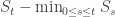
Once we know the structure of the first t vertices, we expect the distribution of X(t) – 1 to be

We aren’t interested in all the edges of the random graph, only in some tree skeleton of each component. So we don’t need to consider the possibility of edges connecting our current location to anywhere we’ve previously visited (as such an edge would have been consider then – it’s a depth-first exploration), hence the -t. But we also don’t want to consider edges connecting our current location to anywhere we’ve seen, since that would be a surplus edge creating a cycle, hence the -S_s. It is binomial because by independence even after all this conditioning, the probability that there’s an edge from my current location to any other vertex apart from those discounted is equal to and independent.

For Mogulskii’s theorem in the previous post, we had an LDP for the rescaled paths of a random walk with independent stationary increments. In this situation we have a random walk where the increments do not have this property. They are not stationary because the pre-limit distribution depends on time. They are also not independent, because the distribution depends on behaviour up to time t, but only through the value of the walk at the present time.

Nonetheless, at least by following through the heuristic of having an instantaneous exponential cost for a LD event, then products of sums becoming integrals within the exponent, we would expect to have a similar result for this case. We can find the rate function latex \text{Po}(\lambda)-1$ and thus get a rate function for paths of the exploration process

where is the height of f above its previous minimum.

Technicalities and Challenges

1) First we need to prove that it is actually possible to extend Mogulskii to this more general setting. Even though we are varying the distribution continuously, so we have some sort of ‘local almost convexity’, the proof is going to be fairly fiddly.

2) Having to consider excursions above the local minima is a massive hassle. We would ideally like to replace with f. This doesn’t seem unreasonable. After all, if we pick a giant component within o(n) steps, then everything considered before the giant component won’t show up in the O(n) rescaling, so we will have a series of macroscopic excursions above 0 with widths giving the actual sizes of the giant components. The problem is that even though with high probability we will pick a giant component after O(1) components, then probability that we do not do this decays only exponentially fast, so will show up as a term in the LD analysis. We would hope that this would not be important – after all later we are going to take an infimum, and since the order we choose the vertices to explore is random and in particular independent of the actual structure, it ought not to make a huge difference to any result.

3) A key lemma in the proof of Mogulskii in Dembo and Zeitouni was the result that it doesn’t matter from an LDP point of view whether we consider the linear (continuous) interpolation or the step-wise interpolation to get a process that actually lives in . In this generalised case, we will also need to check that approximating the Binomial distribution by its Poisson limit is valid on an exponential scale. Note that because errors in the approximation for small values of t affect the parameter of the distribution at larger times, this will be more complicated to check than for the IID case.

4) Once we have a rate function, if we actually want to know about the structure of the ‘typical’ graph displaying some LD property, we will need to find the infimum of the integrated rate function with some constraints. This is likely to be quite nasty unless we can directly use Euler-Lagrange or some other variational tool.

Answer

Papers by O’Connell and Puhalskii have found the rate function. Among other interesting things, we learn that:

while the rate function for the number of edges:

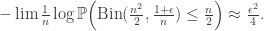
So in fact it looks as if there might be a significant contribution from clustering after all.

Related articles

• New Ramanujan Graphs! (gilkalai.wordpress.com)
• Proof of the Cheeger inequality in manifolds (lucatrevisan.wordpress.com)