Urns and the Dirichlet Distribution

As I’ve explained in some posts from a while ago, I’ve been thinking about some models related to random graph processes, where we ensure the configuration stays critical by deleting any cycles as they appear. Under various assumptions, this behaves in the limit as the number of vertices grows to infinity, like a coagulation-fragmentation process, with multiplicative coalescence and quadratic fragmentation rate, where the fragmentation kernel is the Poisson-Dirichlet distribution, PD(1/2,1/2). I found it quite hard to find accessible notes on these, partly because the theory is still relatively recently, and also because it seems to be one of those topics where you can’t understand anything properly until you kind of understand everything.

This post was motivated and is based on chapter 3 of Pitman’s Combinatorial Stochastic Processes, and the opening pair of lectures from Pierre Tarres’s TCC course on Self-Interaction and Learning.

It makes sense to begin by discussing the Dirichlet distribution, and there to start with the most simple case, the Beta distribution. As we learned in the Part A Statistics course while trying some canonical examples of posterior distributions, it is convenient to ignore the normalising constants of various distributions until right at the end. This is particularly true of the Beta distribution, which is indeed often used as a prior in such situations. The density function of \text{Beta}(\alpha,\beta) is x^{\alpha-1}(1-x)^{\beta-1}. If these are natural numbers, we have a quick proof by induction using integration by parts, otherwise a slightly longer but still elementary argument gives the normalising constant as

\frac{\Gamma(\alpha+\beta)}{\Gamma(\alpha)\Gamma(\beta)}.

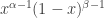
(note that the ‘base case’ is the definition of the Gamma function.) For the generalisation we are about to make, it is helpful to think of this Beta density as a distribution not on [0,1], but on partitions of [0,1] into two parts. That is pairs (x,y) such that x+y=1. Why? Because then the density has the form x^{\alpha-1}y^{\beta-1} and is clear how we might generalise this.

Indeed the Dirichlet distribution with parameters (\alpha_1,\ldots,\alpha_m) is a random variable supported on the subset of \mathbb{R}^m with \sum p_k=1 with density \propto \prod p_k^{\alpha_k-1}. For similar reasons, the correct normalising constant in the general case is

\frac{\Gamma(\sum \alpha_k)}{\prod \Gamma(\alpha_k)}.

You can prove this by inducting on the number of variables, using the Beta distribution as a base case.

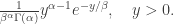
In many situations, it is useful to be able to express some distribution as a function of IID random variables with a simpler distribution. We can’t quite do that for the Dirichlet distribution, but we can express it very simply as function of independent RVs from the same family. It turns out that the family of Gamma distributions is a wise choice. Recall that the gamma distribution with parameters (\alpha,\beta) has density:

\frac{1}{\beta^\alpha \Gamma(\alpha)}y^{\alpha-1}e^{-y/\beta},\quad y>0.

Anyway, define independent RVs Y_k as gamma distributions with parameters (\alpha_k,1), then we can specify (X_1,\ldots,X_m) as the Dirichlet distribution with these parameters by:

(X_1,\ldots,X_m)\stackrel{d}{=}\frac{(Y_1,\ldots,Y_m)}{\sum Y_k}.

In other words, the Dirichlet distribution gives the ratio between independent gamma RVs. Note the following:

– the sum of the gamma distributions, ie the factor we have to scale by to get back to a ratio, is a gamma distribution itself.

– If we wanted, we could define it in an identical way using Gamma with parameters (\alpha_k,\beta) for some fixed \beta.

– More helpfully, because the gamma distribution is additive in the first argument, we can take a limit to construct a gamma process, where the increments have the form required. This will be a useful interpretation when we take a limit, as largest increments will correspond to largest jumps.

Polya’s Urn

This is one of the best examples of a self-reinforcing process, where an event which has happened in the past is more likely to happen again in the future.

The basic model is as follows. We start with one white ball and one black ball in a bag. We draw a ball from the bag uniformly at random then replace it along with an additional ball of the same colour. Repeat this procedure.

The first step is to look at the distribution at some time n, ie after n balls have been added, so there are n+2 in total. Note that there are exactly n+1 possibilities for the state of the bag at this time. We must have between 1 and n+1 black balls, and indeed all of these are possible. In general, part of the reason why this process is self-reinforcing is that any distribution is in some sense an equilibrium distribution.

What follows is a classic example of a situation which is a notational nightmare in general, but relatively straightforward for a fixed finite example.

Let’s example n=5, and consider the probability that the sequence of balls drawn is BBWBW. This probability is:

\frac12\times \frac 23\times \frac14\times \frac 35\times \frac26.

So far this isn’t especially illuminating, especially if we start trying to cancel these fractions. But note that the denominator of the product will clearly be 6!. What about the numerator? Well, the contribution to the numerator of the product from black balls is 1x2x3=3! while the contribution from white balls is 1×2=2!. In particular, the contribution to the numerator from each colour is independent of the order of whites and blacks. It depends only on the number of whites and blacks. So we can conclude that the probability that we end up a particular ordering of k+1 whites and (n-k)+1 blacks is

\frac{k! (n-k)!}{(n+1)!},

and so the probability that we end up with k+1 whites where we no longer care about ordering is

\binom{n}{k}\frac{k!(n-k)!}{(n+1)!}=\frac{1}{n+1}.

In other words, the distribution of the number of white balls in the bag after n balls have been added is uniform on [1, n+1].

That looks like it might be something of a neat trick, so the natural question to ask is what happens if we adjust the initial conditions. Suppose that instead we start with a_1,\ldots,a_m balls of each of m colours. Obviously, this is going to turn into a proof by suggestive notation. In fact, the model doesn’t really rely on the (a_i) being positive integers. Everything carries through with a_i\in\mathbb{R} if we view the vector as the initial distribution.

As before, the order in which balls of various colours are drawn doesn’t matter hugely. Suppose that the first n balls drawn feature n_i balls of colour i. The probability of this is:

\binom{n}{n_1,\ldots,n_k}\frac{\prod_i \alpha_i(\alpha_i+1)\ldots (\alpha_i+n_i-1)}{\alpha(\alpha+1)\ldots(\alpha+(n-1))}

where \alpha=\sum_i \alpha_i. Then for large n, assuming for now that the \alpha_i\in\mathbb{N} we have

\frac{\alpha(\alpha+1)\ldots(\alpha+n-1)}{n!}=\frac{[\alpha_i+(n_i-1)]!}{n_i! (\alpha_i-1)!}\approx \frac{n_i^{\alpha_i-1}}{(\alpha_i-1)!}.

The denominator will just be a fixed constant, so we get that overall, the probability above is approximately

\frac{\prod_i n_i^{\alpha_i-1}}{n^{\alpha-1}}=\prod (\frac{n_i}{n})^{\alpha_i-1},

which we recall is the pdf of the distribution distribution with parameters (\alpha_i) as telegraphed by our choice of notation. With some suitable martingale machinery, you can also prove that this convergence happens almost surely, for a suitable limit RV defined on the tail sigma algebra.

Next time I’ll introduce a more complicated family of self-reinforcing processes, and discuss some interesting limits of the Dirichlet distribution that relate to such processes.

Enhanced by Zemanta

Bayesian Inference and the Jeffreys Prior

Last term I was tutoring for the second year statistics course in Oxford. This post is about the final quarter of the course, on the subject of Bayesian inference, and in particular on the Jeffreys prior.

There are loads and loads of articles sitting around on the web contributing the debate about the relative merits of Bayesian and frequentist methods. I do not want to continue that debate here, partly because I don’t have a strong opinion, but mainly because I don’t really understand that much about the underlying issues.

What I will say is that after a few months of working fairly intensively with various complicated stochastic processes, I am starting to feel fairly happy throwing about conditional probability rather freely. When discussing some of the more combinatorial models for example, quite often we have no desire to compute or approximate complication normalising constants, and so instead talk about ‘weights’. And a similar idea underlies Bayesian inference. As in frequentist methods we have an unknown parameter, and we observe some data. Furthermore, we know the probability that such data might have arisen under any value of the parameter. We want to make inference about the value of the parameter given the data, so it makes sense to multiply the probability that the data emerged as a result of some parameter value by some weighting on the set of parameter values.

In summary, we assign a prior distribution representing our initial beliefs about the parameter before we have seen any data, then we update this by weighting by the likelihood that the observed data might have arisen from a particular parameter. We often write this as:

\pi(\theta| x)\propto f(x|\theta)\pi(\theta),

or say that posterior = likelihood x prior. Note that in many applications it won’t be necessary to work out what the normalising constant on the distribution ought to be.

That’s the setup for Bayesian methods. I think the general feeling about the relative usefulness of such an approach is that it all depends on the prior. Once we have the prior, everything is concrete and unambiguously determined. But how should we choose the prior?

There are two cases worth thinking about. The first is where we have a lot of information about the problem already. This might well be the case in some forms of scientific research, where future analysis aims to build on work already completed. It might also be the case that we have already performed some Bayesian calculations, so our current prior is in fact the posterior from a previous set of experiments. In any case, if we have such an ‘informative prior’, it makes sense to use it in some circumstances.

Alternatively, it might be the case that for some reason we care less about the actual prior than about the mathematical convenience of manipulating it. In particular, certain likelihood functions give rise to conjugate priors, where the form of the posterior is the same as the form of the prior. For example, a normal likelihood function admits a normal conjugate prior, and a binomial likelihood function gives a Beta conjugate prior.

In general though, it is entirely possible that neither of these situations will hold but we still want to try Bayesian analysis. The ideal situation would be if the choice of prior had no effect on the analysis, but if that were true, then we couldn’t really be doing any Bayesian analysis. The Jeffreys prior is one natural candidate because it removes a specific problem with choosing a prior to express ignorance.

It sounds reasonable to say that if we have total ignorance about the parameter, then we should take the prior to be uniform on the set of possible values taken by the parameter. There are two potential objections to this. The first is that if the parameter could take any real value, then the prior will not be a distribution as the uniform distribution on the reals is not normalisable. Such a prior is called improper. This isn’t a huge problem really though. For making inference we are only interested in the posterior distribution, and so if the posterior turns out to be normalisable we are probably fine.

The second problem is more serious. Even though we want to express ignorance of the parameter, is there a canonical choice for THE parameter? An example will make this objection more clear. Suppose we know nothing about the parameter T except that it lies in [0,1]. Then the uniform distribution on [0,1] seems like the natural candidate for the prior. But what if we considered T^100 to be the parameter instead? Again if we have total ignorance we should assign T^100 the uniform distribution on its support, which is again [0,1]. But if T^100 is uniform on [0,1], then T is massively concentrated near 1, and in particular cannot also be uniformly distributed on [0,1]. So as a minimum requirement for expressing ignorance, we want a way of generating a prior that doesn’t depend on the choice of parameterisation.

The Jeffreys prior has this property. Note that there may be separate problems with making such an assumption, but this prior solves this particular objection. We define it to be \pi(\theta)\propto [I(\theta)]^{1/2} where I is the Fisher information, defined as

I(\theta)=-\mathbb{E}_\theta\Big[\frac{\partial^2 l(X_1,\theta)}{\partial \theta^2}\Big],

where the expectation is over the data X_1 for fixed \theta, and l is the log-likelihood. Proving that this has the property that it is invariant under reparameterisation requires demonstrating that the Jeffreys prior corresponding to g(\theta) is the same as applying a change of measure to the Jeffreys prior for \theta. The proof is a nice exercise in the chain rule, and I don’t want to reproduce it here.

For a Binomial likelihood function, we find that the Jeffreys prior is Beta(1/2,1/2), which has density that looks roughly like a bucket suspended above [0,1]. It is certainly worth asking why the ‘natural’ choice for prior might put lots of mass at the edge of the domain for the parameter.

I don’t have a definitive answer, but I do have an intuitive idea which comes from the meaning of the Fisher information. As the second derivative of the log-likelihood, a large Fisher information means that with high probability we will see data for which the likelihood changes substantially if we vary the parameter. In particular, this means that the posterior probability of a parameter close to 0 will be eliminated more quickly by the data if the true parameter is different.

If the variance is small, as it is for parameter near 0, then the data generated by this parameter will have the greatest effect on the posterior, since the likelihood will be small almost everywhere except near the parameter. We see the opposite effect if the variance is large. So it makes sense to compensate for this by placing extra prior mass at parameter values where the data has the strongest effect. Note that in the previous example, the Jeffreys prior is in fact exactly inversely proportional to the standard deviation. For the above argument to make sense, we need it to be monotonic with respect to SD, and it just happens that in this case, being 1/SD is precisely the form required to be invariant under reparameterisation.

Anyway, I thought that was reasonably interesting, as indeed was the whole course. I feel reassured that I can justify having my work address as the Department of Statistics since I now know at least epsilon about statistics!