Linear Algebra II: Eigenvectors and Diagonalisability

This post continues the discussion of the Oxford first-year course Linear Algebra II. We’ve moved on from determinants, and are now considering eigenvalues and eigenvectors of matrices and linear maps.

A good question to ask is: what’s the point of knowing about eigenvectors? I can think of a quick answer and a longer answer. The quick answer is that whenever we have a mapping of any kind, it is natural to ask about its fixed points. And since we are thinking about vector spaces and linear maps, if we can’t find any fixed points, we might nonetheless be able to find the best thing, some vectors whose direction is fixed by the map. In general, knowing about fixed points of a mapping might tell us other more qualitative properties, including the behaviour seen when you apply the map iteratively a large number of times. (Indeed a recent post discusses this exact problem for positive matrices in a context relevant to a chapter of my thesis…)

A more specific answer concerns bases. Recall that a linear map is defined independently of any basis: it’s just a map from the vector space to itself. We can express the linear map via a matrix with respect to some basis, but how to choose the basis? We could always choose the canonical basis in , since it’s easy to do vector and matrix calculations when most of the entries of all the vectors are zero. We also have a good visual idea (at least in up to three dimensions) of what a matrix might mean with respect to that basis. If we needed to divide the three-dimensional world around us into small volumes, we’d tend to describe it with small cubes rather than small arbitrary parallelopipeds.

But once we know something about the linear map, we might want to choose a basis of vectors on which the behaviour of the map is particularly easy to describe. And eigenvectors fulfil precisely this role. If we are able to choose a basis of eigenvectors, describing the map’s action, either abstractly, or via a (diagonal) matrix, is very straightforward. If we are given a matrix to begin with, we know how to do a change of basis, and changing to the basis of eigenvectors is precisely what’s going when we write , where D is a diagonal matrix. We construct P by taking its columns to be these eigenvectors. In particular, for a given vector x, y=Px is the vector giving the coefficients of x in the basis of eigenvectors.

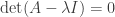
So the case where we have a basis of eigenvectors is particularly useful, and in this case, we say the matrix or the map is diagonalisable. Remember how we find eigenvalues. If there exists a non-zero vector x satisfying , then x is in the kernel of . As we discussed last time, introducing the determinant gives a much more manageable way to verify which values of result in having a non-trivial kernel. In particular, if non-zero x is in the kernel, we have , and this leads to a polynomial of degree n (the dimensional of the vector space / size of the matrix) for , called the characteristic polynomial , which has the eigenvalues as its roots.

If we agree to work over the complex field, then this is good, because it means we always have eigenvalues, and so it becomes sensible to talk about exactly how many eigenvalues and eigenvectors we have. Observe that if we restrict to real vector spaces, this might not be the case. In the plane, the rotation by for example has no fixed vectors.

Multiplicities of eigenvalues

We call the algebraic multiplicity of an eigenvalue to be the exponent of the factor in the factorisation of the characteristic polynomial. To define the geometric multiplicity, observe that all the eigenvectors with eigenvalue form a subspace, and so it is meaningful to talk about the dimension of this subspace (‘eigenspace’), which is the geometric multiplicity . There are two facts that one needs to remember. The slightly less obvious one is that for all . One can see this by, for example, working in a basis that extends a basis of the -eigenspace. Observe at this stage that the sum of the algebraic multiplicities has to be n by definition, while the sum of geometric multiplicities is at most n. And this makes sense, because the space spanned by all the eigenvectors is a subspace, and so has dimension at most n.

The more obvious, but more frequently forgotten result is that

which is simply a consequence of the property discussed a few paragraphs previously concerning the kernel of .

In particular, we might make the heuristic observation that ‘most’ polynomials of degree n have n distinct roots. This is certainly true for quadratics: there is only one value that the discriminant can take such that we see a repeated root. Alternatively, imagine shifting the quadratic up and down (in a complex way if necessary); again there is only one moment at which it might have a repeated root. This observation can be generalised easily to higher degree polynomials in a number of ways.

So if we lift this observation across to matrices, we see that most matrices have n distinct eigenvalues, and thus have n linearly independent eigenvectors which form a basis, hence the matrix is diagonalisable. I think it’s really worth reflecting on this, since much of a first exploration into linear algebra ends up treating exactly the case where the matrix is not diagonalisable.

The principal example of a non-diagonalisable matrix is , where the 2s can be replaced by any value, and the 1 can be replaced by an non-zero value. There’s plenty to learn about to what extent versions of this matrix of higher size represent all non-diagonalisable matrices, but such an exposition of Jordan normal form comes next year for the students taking this course.

It probably is worth saying now though, that this example gives a good sanity check for whether a method is actually using diagonalisability correctly. For example, it is easily seen that elementary row operations to not preserve diagonalisability by starting from and ending up at our counter-example. One could also argue from this that the set of non-diagonalisable matrices are dense within the set of matrices with a repeated eigenvalue. That is, having a repeated eigenvalue but full eigenspace is doubly-infinitely-unlikely.

Cayley-Hamilton theorem

Anyway, among other results, we also saw the Cayley-Hamilton theorem, which states that a matrix A satisfies its own characteristic equation. That is , where the zero on the right-hand side is the zero matrix. It’s tempting to substitute A into the expression , but of course this is not valid. Indeed imagine a typical eigenvalue determinant matrix with terms like on the diagonal; it doesn’t make sense to substitute a matrix for as one of the entries of the overall matrix!

Fortunately, we can argue convincingly in the case where A is a diagonalisable matrix. Remember that is a matrix. Now looki at the action of on any eigenvector v, corresponding to eigenvalue . Applying some power of A to v gives v multiplied by the same power of , and so we end up with

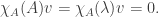
This only worked when v was an eigenvector, but fortunately there is a basis of eigenvectors if A is diagonalisable, and so for all v, hence .

But is just a matrix-valued function of A. If you think about it, is a monic polynomial, all of whose non-leading coefficients are multinomials of degree at most n-1 in the entries of A. Furthermore, these multinomials have (non-negative) integer coefficients. Therefore the entries of are multinomials of degree at most 2n-1 in the entries of A, and again have (non-negative) integer coefficients.

Even without the integrality of the coefficients, this says that, under any reasonable definition of continuity of matrices (which could be induced from any topology on ) the function should be continuous as a function of A. But we’ve shown for all diagonalisable A, and also argued that most complex-valued matrices are diagonalisable. Turning this into a formal statement about denseness means that we’ve shown the Cayley-Hamilton theorem for non-diagonalisable matrices also. It feels that because the coefficients are non-negative integers, we might also have shown the result for other fields too, but I have minimal knowledge or recollection at the moment of the things one has to check for this sort of result.

It’s worth ending with the brief comment that Cayley-Hamilton is useful, among other reasons because it enables us to write the inverse of A as a polynomial of degree at most n-1 in terms of A. In many settings this is a lot easier to work with in terms of calculations than an argument with minors.

Linear Algebra II: Determinants 2

In the previous post, we introduced determinants of matrices (and by extension linear maps) via its multilinearity properties, and as the change-of-volume factor. We also discussed how to calculate them, via row operations, or Laplace expansion, or directly via a sum of products of entries over permutations.

The question of why this is ever a useful quantity to consider remains, and this post tries to answer it. We’ll start by seeing one example where this is a very natural quantity to consider, and then the main abstract setting, where the determinant is zero, and consider a particularly nice example of this.

Jacobeans as a determinant

We consider integration by substitution. Firstly, in one variable: when it comes to Riemann integration of a function g(x) with respect to x, we view dx as the width of a small column which approximates the function near x. Now, if we reparameterise, that is if we write x=f(y) for some well-behaved (in particular differentiable) function f, then the width of the column is dx= dy.(dx/dy)=f'(y) dy. This may be negative, if y is decreasing while x is increasing, but for now let’s not worry about this overly, for example by assuming the function g is non-negative. Thus if we want to integrate with y as the variable, we multiply the integrand by this factor .

What about in higher dimensions? We have exactly the same situation, only instead of two-dimensional columns, we have (n+1)-dimensional columns. We then multiply the n-dimensional volume of the base by the height, again given by . If we have a similar transformation of the base variable , we differentiate to get

In other words

where J is the Jacobean matrix of partial deriatives. In particular, we know how to relate the volume to the volume . It’s simply the determinant of the Jacobean J. So if we want to integrate with respect to , it only remains to pre-multiply the integrand by and proceed otherwise as in the one-dimensional case.

Det A = 0

A first linear algebra course might well motivate the introducing matrices as a notational shortcut for solving families of linear equations, . The main idea is that generally we can solve this equation uniquely. Almost all of the theory developed in such a first linear algebra course deals with the case when this fails to hold. In particular, there are many ways to characterise this case, and we list some of them now:

• Ax=b has no solutions for some b;
• A is not invertible;
• A has non-trivial kernel, that is, with dimension at least one;
• A does not have full rank, that is, the image has dimension less than n;
• The columns (or indeed the rows) are linearly dependent;
• The matrix can be row-reduced to a matrix with a row of zeroes.

It is useful that these are equivalent, as in abstract problems one can choose whichever interpretation from this list is most relevant. However, all of these are quite hard to check. Exhibiting a non-trivial kernel element is hard – one either has to do manual row-reduction, or the equivalent in the context of linear equations. But we can add the characterisation

• det A = 0;

to the list. And this is genuinely much easier to check for specific examples, either abstract or numerical.

Let’s quickly convince ourselves of a couple of these equivalences. Determinant is invariant under row-reductions, and by multilinearity it is certainly the case that det A = 0 if A has a row of zeroes. We also said that A is the change-of-volume factor. Note that A is a map from the domain to its image, so if A has less than full rank, then any set in the image has zero volume.

The Vandermonde matrix

This is a good example of this theory in practice. Consider the Vandermonde matrix where each row is a geometric progression:

Now suppose we attempt to solve

There’s a natural interpretation to this, that’s especially clear with this suggestive notation. Each row corresponds to a polynomial, where the coefficients are given by the , and the argument is given by .

So if we try to solve for , given and , we are asking whether we can find a polynomial P with degree at most n-1 such that for . Lagrange interpolation gives an argument where we just directly write down the relevant polynomial, but we can also deploy our linear algebraic arguments too.

The equivalence of all these statements means that to verify existence and uniqueness of such a polynomial, we only need to check that the Vandermonde matrix has non-zero determinant. And in fact there are a variety of methods to show that

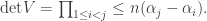
For the polynomial question to be meaningful, we would certainly demand that the are distinct, and so this determinant is non-zero, and we’ve shown that n points determine a degree (n-1) polynomial uniquely.

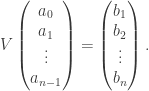
If we multiply on the left instead, suppose that we are considering a discrete probability distribution X that takes n known values with unknown probabilities . Then we have

So, again by inverting the Vandermonde matrix (which is know is possible since its determinant is non-zero…) we can recover the distribution from the first (n-1) moments of the distribution.

A similar argument applies to show that the Discrete Fourier Transform is invertible, and in this case (where the s are roots of unity), the expression for the Vandermonde determinant is particularly tractable.

Linear Algebra II: Determinants 1

This term, I’m giving tutorials on a course that’s new to me, the apparently notorious ‘Linear Algebra II’ for first year undergraduates. I can appreciate how it might have ended up with this reputation, but as always, every challenge is also an opportunity, So I’m going to (try to) write a short series of blog posts about what we’ve discussed in the tutorials.

The first problem sheet-and-a-half concerned determinants of matrices. There are three things worth addressing here:

1. What are abstract definitions, and which is most useful in each setting?
2. How to actually calculate them?
3. What’s the overall point?

The answers are obviously not completely unrelated, but we’ll probably defer the third question to a second post.

The determinant is a map from the set of matrices to the base field (hereafter assumed to be ). The Oxford course defines it through its properties:

• Multilinear in the columns of the matrix.
• Equal to zero if two columns are equal.
• Equal to one if the matrix is the identity.

One then checks that there is a unique such map, and so from now on it’s reasonable to call it the determinant of the matrix. It will follow from pretty much any consequence that we can replace ‘columns’ with ‘rows’ throughout and get the same map.

Other definitions

We have a closed form expression for the determinant given via permutations of n

We’ll come back to a discussion of when this particular definition is useful. It can be derived by carefully transforming the identity matrix into A, using the operations which are mentioned in the original definition of the determinant, in particular, keeping track of the number of transpositions of columns.

It’s clear from any definition that the determinant is a polynomial of degree n in the entries of the matrix, but this definition will be useful if you want to make some more precise comment on the nature of this polynomial. For example, if entries of the matrix are polynomials in x of various degree (think of the eigenvalue equation for example) this allows you to control (or at least bound) the overall degree of the determinant as a polynomial in x.

The determinant is also the volume of the n-dimensional parallelopiped formed by the column vectors of the matrix. This is easy to check in two dimensions, for the matrix :

To calculate the area of the central parallelogram, we have to subtract the area of two small rectangles and four small triangles from the outer rectangle, obtaining

as we expect. This calculation is harder to execute in higher dimensions, and certainly harder to visualise.

Maybe, though, we don’t have to, so long as we can reassure ourselves that this volume satisfies the implicit definition of the determinant map at the start. Multilinearity in the columns is not that hard to see. If we multiply the jth column by some constant, we are stretching the parallelopiped by the same constant factor in one direction, and so the volume grows appropriately. The additivity property can similarly be thought of as joining together two parallelopipeds at their common face (which is common since the other column vectors have to be constant in this construction). If two column vectors are equal, then clearly this volume actually has dimension at most n-1, and thus volume zero, so the final two conditions are genuinely easy to check.

The challenge here is that there is a direction involved. Determinants can be negative, but in our classical viewpoint, areas generally are not. In 2D, we can think of this as saying that the area is positive if the vector (b,d) lies anti-clockwise from (a,c) in the parallelogram, while is it negative otherwise. Again, this is harder to visualise in higher dimensions, but it is at least plausible that one could develop a similar decomposition. Ultimately, we are happy with the notion of directed lengths (ie vectors on the real line), and these are easy to add up without having to separate into cases, and the case holds for areas and higher-dimensional volumes.

Evaluating determinants

If we actually want to compute the determinant of a given matrix, the sum over permutations is intractable since it doesn’t have any natural splits into stages. The implicit definitions and this area consideration are clearly useless for all but the most special of examples.

The Laplace expansion is the usual algorithm to calculate the determinant of an n x n matrix. You pick a row (or a column), and evaluate the determinants of the (n-1) x (n-1) minor matrices given by deleting this row (or column), and each column (or row) in turn. This leaves us with n determinants of smaller matrices, which we pre-multiply by the entries in the original deleted row (or column), and add up in an alternating way (*). This is highly computationally intensive for large matrices, but for 3×3 and 4×4 can be done by hand with probability of an error bounded away from 1.

There is the flexibility to choose the reference row or column. Since the entries of these affect the sum through small products, it is highly convenient to choose a row or column with a lot of zeros. In particular, if there’s a row or column with exactly one non-zero entry, this is an ideal candidate.

The sum over permutations also works well when a lot of the entries are zero, because then a lot of the permutations give a summand which is zero. Upper-triangular matrices are a good example: only one permutation (the identity permutation) avoids all the zero elements underneath the diagonal.

One can also observe from the multilinearity property of the determinant map that there are lots of operations we can apply to the matrix which leave the determinant fixed. These are often called elementary row operations, though obviously we can apply them to the columns as well. To summarise, if we interchange two rows, the sign of the determinant is reversed. And if we add some multiple of one row to any other row, the determinant stays the same.

When matrices are not square, it’s quite important to be specific about exactly what form you can reduce a general matrix to via such row operations, but in this context, it’s not hugely important. Reduced echelon form (without the condition that leading coefficients will be one) is achievable, but this is a special case of an upper triangular matrix, for which the determinant is given by the product of the diagonal entries, ie is easy.

Whether this is substantially easier than Laplace expansion depends on the matrix itself and taste, both to do manually, and to code.

(*) I’m not a fan personally of this alternating definition. It seems to me much more natural to define the minor as

with indices taken modulo n. Then you don’t have any s in the Laplace expansion.

Using determinants in abstract problems

So the determinant gives directly the area of the image (under A) of the unit hypercube. By linearity (of A), it is easy to see that it also gives the scale factor of the area change (under A) of any hyper-cuboid, parallel to the conventional axes, anywhere in the space. Then, eg by approximating any sensible n-dimensional shape (*) as a union of such hyper-cuboids, we can show that in fact the area of any sensible shape increases by a factor (det A) under application of A.

This is a good thing to remember, because it is an excellent heuristic for seeing why the determinant of a linear map is basis-independent. It also gives a much easier proof of the key result

than that given by fixing B and viewing det(AB) as a map from matrices to the field, just like the original definition of determinant.

Some of the theory in the course is proved using elementary row operations. But these invite complicated notation, so are best used only in simple arguments, or when things are fairly explicit to begin with. Given an abstract problem about determinants of matrices, it is often tempting to induct on the size of the matrix in some way. I think it’s worth saying that even though the Laplace expansion is explicitly set up in this way, the notation involved is also likely to be annoying here, while permutations are easy to describe inductively: eg let , then view the remainder of the permutation as a bijection .

Shortly, we’ll have a second post answering the final question: what’s the point of working with determinants? We’ve already seen half an answer, in that they describe the change-of-volume factor of a matrix (or linear map), but this can be substantially developed.