enumerative combinatorics | Eventually Almost Everywhere

I’ve just got back from a visit to Budapest University of Technology, where it was very pleasant to be invited to give a talk, as well as continuing the discussion our research programme with Balazs. My talk concerned a limit for the exploration process of an Erdos-Renyi random graph conditioned to have no cycles. Watch this space (hopefully very soon) for a fully rigorous account of this. In any case, my timings were not as slick as I would like, and I had to miss out a chunk I’d planned to say about a result of Britikov concerning enumerating unrooted forests. It therefore feels like an excellent time to write something again, and explain this paper, which you might be able to find here, if you have appropriate journal rights.

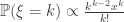
We are interested to calculate $a_{n,m}$ the number of forests with vertex set [n] consisting of m unrooted trees. Recall that if we were interested in rooted trees, we could appeal to Prufer codes to show that there are $m n^{n-m-1}$ such forests, and indeed results of Pitman give a coalescent/fragmentation scheme as m varies between 1 and n-1. It seems that there is no neat combinatorial re-interpretation of the unrooted case though, so Britikov uses an analytic method.

We know that

$a_{n,m}= \frac{n!}{m!} \sum_{\substack{k_1+\ldots+k_m=n\\ k_i\ge 1}} \prod_{j=1}^m \frac{k_j^{k_j-2}}{k_j!}.$

To see this, observe that the $k_j$ s correspond to the sizes of the m trees in the forest; $\frac{n!}{\prod k_j!}$ gives the multinomial number of ways to assign vertices to the trees; given the labels for a tree of size $k_j$ , there are $k_j^{k_j-2}$ ways to make up the tree itself; and $\frac{1}{m!}$ accounts for the fact that the trees have no order.

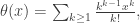
What we would really like to do is to take the uniform distribution on the set of all labelled trees, then simulate m IID copies of this distribution, and condition the union to contain precisely n vertices. But obviously this is an infinite set, so we cannot choose uniformly from it. Instead, we can tilt so that large trees are unlikely. In particular, for each x we define

$\mathbb{P}(\xi=k) \propto \frac{k^{k-2} x^k}{k!}$ ,

and define the normalising constant

$B(x):= \sum_{k\ge 1} \frac{k^{k-2}x^k}{k!},$

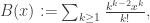
whenever it exists. It turns out that $x\le e^{-1}$ is precisely the condition for $B(x)<\infty$ . Note now that if $\xi_1,x_2,\ldots$ are IID copies of $\xi$ , then

$\mathbb{P}(\xi_1+\ldots+\xi_m=n) = \frac{x^n}{B(x)^m} \sum_{k_1+\ldots + k_m=n} \prod_{j=1}^m \frac{k_j^{k_j-2}}{k_j!},$

and so we obtain

$a_{n,m}= \frac{n!}{m!} \frac{B(x)^m}{x^n} \mathbb{P}(\xi_1+\ldots + \xi_m=n).$

So asymptotics for $a_{n,m}$ might follows from laws of large numbers of this distribution $\xi$ .

So far, we haven’t said anything about how to choose this value x. But observe that if you want to have lots of trees in the forest, then the individual trees should generally be small, so we take x small to tilt away from a preference for large trees. It turns out that there is a similar interpretation of criticality for forests as for general graphs, and taking x equal to 1/e, its radius of convergence works well for this setting. If you want even fewer trees, there is no option to take x larger than 1/e, but instead one can use large deviations machinery rather than laws of large number asymptotics.

We will be interested in asymptotics of the characteristic function of $\xi$ for x=1/e. In particular $\mathbb{E}[e^{it\xi}]=\frac{B(xe^{it})}{B(x)}$ , and it will be enough to clarify the behaviour of this as $t\rightarrow 0$ . It’s easier to work with a relation analytic function

$\theta(x)=\sum_{k\ge 1} \frac{k^{k-1}x^k}{k!},$

ie the integral of B. What now feels like a long time ago I wrote a masters’ thesis on the subject of multiplicative coalescence, and this shows up as the generating function of the solutions to Smoluchowski’s equations with monodisperse initial conditions, which are themselves closely related to the Borel distributions. In any case, several of the early papers on this topic made progress by establishing that the radius of convergence is 1/e, and that 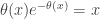$\theta(x)e^{-\theta(x)}=x$ everywhere where $|x|\le 1/e$ . We want to consider x=1/e, for which $\theta=1$ .

Note that $\mathbb{E}\xi = \frac{\theta(x)}{B(x)}$ , so we will make progress by relating $B(x),\theta(x)$ in two ways. One way involves playing around with contour integrals in a fashion that is clear in print, but involves quite a lot of notation. The second way is the Renyi relation which asserts that $\theta(x)=B(x)+\frac{\theta(x)^2}{2}$ . We will briefly give a combinatorial proof. Observe that after multiplying through by factorials and interpreting the square of a generating function, this is equivalent to

$k^{k-1} = k^{k-2} + \frac12 \sum_{\substack{l+m=k\\l,m\ge 1}} l^{l-1}m^{m-1}\binom{k}{l},$

for all k. As we might expect from the appearance of this equality, we can prove it using a bijection on trees. Obviously on the LHS we have the size of the set of rooted trees on [k]. Now consider the set of pairs of disjoint rooted trees with vertex set [k]. This second term on the RHS is clearly the size of this set. Given an element of this set, join up the two roots, and choose whichever root was not initially in the same tree as 1 to be the new root. We claim this gives a bijection between this set, and the set of rooted trees on [k], for which 1 is not the root. Given the latter, the only pair of trees that leads to the right rooted tree on [k] under this mapping is given by cutting off the unique edge incident to the root that separates the root and vertex 1. In particular, since there is a canonical bijection between rooted trees for which 1 is the root, and unrooted trees (!), we can conclude the Renyi relation.

The Renyi relation now gives $\mathbb{E}\xi = \frac{\theta(x)}{B(x)}=2$ when x=1/e. If we wanted, we could show that the variance is infinite, which is not completely surprising, as the parameter x lies on the radius of convergence of the generating function.

Now, playing around with contour integrals, and being careful about which strands to take leads to the asymptotic as $t\rightarrow 0$

$\mathbb{E}[ e^{it\xi}] = 1+2it + \frac{2}{3}i |2t|^{3/2} (i\mathrm{sign}(t))^{3/2} + o(|t|^{3/2}).$

So from this, we can show that the characteristic function of the rescaled centred partial sum $\frac{\xi_1+\ldots+\xi_N-2N}{bN^{2/3}}$ converges to $\exp(-|t|^{3/2}\exp(\frac{i\pi}{4}\mathrm{sign} t))$ , where $b= (32/9)^{1/3}$ is a constant arising out of the previous step.

We recognise this as the characteristic function of the stable distribution with parameters 3/2 and -1. In particular, we know now that $\xi$ is in the domain of attraction for a stable-3/2 distribution. If we wanted a version of the central limit theorem for such partial sums, we could have that, but since we care about the partial sums of the $\xi_i$ s taking a specific value, rather than a range of values on the scale of the fluctuations, we actually need a local limit theorem.

To make this clear, let’s return to the simplest example of the CLT, with some random variables with mean $\mu$ and variance $\sigma^2<\infty$ . Then the partial sums satisfy

$\mathbb{P}(\mu N + a\sigma\sqrt{N} \le S_N \le \mu_N+b\sigma\sqrt{N}) \rightarrow \int_a^b f_{\mathcal N}(x)dx,$

as $N\rightarrow\infty$ . But what about the probability of $S_N$ taking a particular value m that lies between $\mu N+a\sigma \sqrt{N}$ and $\mu N + b\sigma \sqrt{N}$ ? If the underlying distribution was continuous, this would be uncontroversial – considering the probability of lying in a range that is smaller than the scale of the CLT can be shown in a similar way to the CLT itself. A local limit theorem asserts that when the underlying distribution is supported on some lattice, mostly naturally the integers, then these probabilities are in the limit roughly the same whenever m is close to $\mu N+a\sigma\sqrt{N}$ .

In this setting, a result of Ibragimov and Linnik that I have struggled to find anywhere in print (especially in English) gives us local limit theory for integer-supported distributions in the domain of attraction of a stable distribution. Taking p( ) to be the density of this distribution, we obtain

$bm^{2/3}\mathbb{P}(\xi_1+\ldots+\xi_m=n) - p(\frac{n-2m}{b m^{2/3}}) \rightarrow 0$

as $n\rightarrow\infty$ , uniformly on any set of m for which $z= \frac{n-2m}{bm^{2/3}}$ is bounded. Conveniently, the two occurrences of b clear, and Britikov obtains

$a_{n,m} = (1+o(1)) \frac{\sqrt{2\pi} n^{n-1/6}}{2^{n-m}(n-m)!} p(\frac{n-2m}{n^{2/3}},$

uniformly in the same sense as before.

Eventually Almost Everywhere

A blog about probability and olympiads by Dominic Yeo

Tag Archives: enumerative combinatorics

Enumerating Forests